机器学习之贝叶斯算法图像分类

article/2025/10/15 22:10:44

在这里插入图片描述
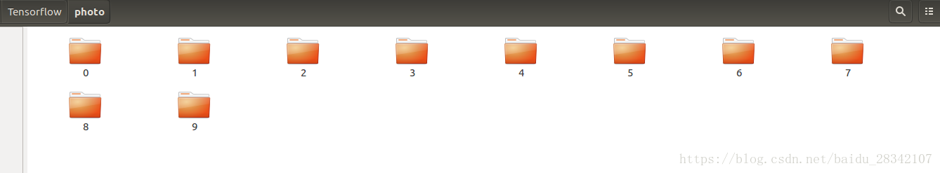
数据集：数据集采用Sort_1000pics数据集。数据集包含1000张图片，总共分为10类。分别是人(0)，沙滩（1），建筑（2），大卡车（3），恐龙（4），大象（5），花朵（6），马（7），山峰（8），食品（9）十类，每类100张，（数据集可以到网上下载）。
在这里插入图片描述
ubuntu16.04虚拟操作系统，在分配内存4G,处理器为1个CPU下的环境下运行。
将所得到的图片至“./photo目录下”，（这里采用的是Anaconda3作为开发环境）。可以参考上一篇
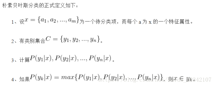
伯努利分布理论基础：
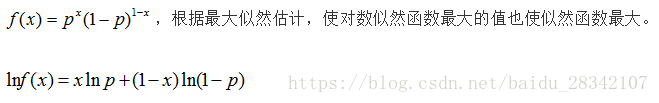
该分布研究的是一种特殊的实验，这种实验只有两个结果要么成功要么失败，且每次实验是独立的并每次实验都有固定的成功概率p。用伯努利朴素贝叶斯实现对图像的分类，首先伯努利分类对象是0,1分类，故此需要将图像像素进行阈值0,1划分。
在这里插入图片描述

import datetime
starttime = datetime.datetime.now()import numpy as np
from sklearn.cross_validation import train_test_split
from sklearn.metrics import confusion_matrix, classification_report
import os
import cv2X = []
Y = []for i in range(0, 10):#遍历文件夹，读取图片for f in os.listdir("./photo/%s" % i):#打开一张图片并灰度化Images = cv2.imread("./photo/%s/%s" % (i, f)) image=cv2.resize(Images,(256,256),interpolation=cv2.INTER_CUBIC)hist = cv2.calcHist([image], [0,1], None, [256,256], [0.0,255.0,0.0,255.0]) X.append(((hist/255).flatten()))Y.append(i)
X = np.array(X)
Y = np.array(Y)
#切分训练集和测试集
X_train, X_test, y_train, y_test = train_test_split(X, Y, test_size=0.3, random_state=1)
#随机率为100%（保证唯一性可以对比）选取其中的30%作为测试集from sklearn.preprocessing import binarize 
from sklearn.preprocessing import LabelBinarizerclass ML:def predict(self, x):#预测标签X = binarize(x, threshold=self.threshold)#使对数似然函数最大的值也使似然函数最大#Y_predict = np.dot(X, np.log(prob).T)+np.dot(np.ones((1,prob.shape[1]))-X, np.log(1-prob).T)#等价于  lnf(x)=xlnp+(1-x)ln(1-p)Y_predict = np.dot(X, np.log(self.prob).T)-np.dot(X, np.log(1-self.prob).T) + np.log(1-self.prob).sum(axis=1)return self.classes[np.argmax(Y_predict, axis=1)]class Bayes(ML): def __init__(self,threshold):self.threshold = thresholdself.classes = []self.prob = 0.0def fit(self, X, y):#标签二值化labelbin = LabelBinarizer()Y = labelbin.fit_transform(y) self.classes = labelbin.classes_ #统计总的类别，10类Y = Y.astype(np.float64)#转换成二分类问题X = binarize(X, threshold=self.threshold)#特征二值化,threshold阈值根据自己的需要适当修改feature_count = np.dot(Y.T, X) #矩阵转置，对相同特征进行融合class_count = Y.sum(axis=0) #统计每一类别出现的个数#拉普拉斯平滑处理，解决零概率的问题alpha = 1.0smoothed_fc = feature_count + alphasmoothed_cc = class_count + alpha * 2self.prob = smoothed_fc/smoothed_cc.reshape(-1, 1)return selfclf0 = Bayes(0.2).fit(X_train,y_train) #0.2表示阈值
predictions_labels = clf0.predict(X_test)
print(confusion_matrix(y_test, predictions_labels))
print (classification_report(y_test, predictions_labels))
endtime = datetime.datetime.now()
print (endtime - starttime)

实验结果为：

[[20  0  0  0  0  1  0 10  0  0][ 1  2  5  0  0  0  0 23  0  0][ 3  0  9  0  1  0  0 13  0  0][ 0  0  1 18  0  1  1  5  0  3][ 0  0  0  0 30  1  0  0  0  1][ 0  0  0  0  1  6  0 26  0  1][ 3  0  0  2  0  0 21  3  0  1][ 0  0  0  0  0  0  0 26  0  0][ 2  0  0  2  1  1  0 21  2  2][ 2  0  2  3  1  0  1 15  0  6]]precision    recall  f1-score   support0       0.65      0.65      0.65        311       1.00      0.06      0.12        312       0.53      0.35      0.42        263       0.72      0.62      0.67        294       0.88      0.94      0.91        325       0.60      0.18      0.27        346       0.91      0.70      0.79        307       0.18      1.00      0.31        268       1.00      0.06      0.12        319       0.43      0.20      0.27        30avg / total       0.70      0.47      0.45       3000:00:05.261369

大家可根据自己的数据集图像，调整划分阈值，可以得到不同的分类精度。代码参考了from sklearn.naive_bayes import BernoulliNB里面的代码。下面贴出集成的代码：

import datetime
starttime = datetime.datetime.now()import numpy as np
from sklearn.cross_validation import train_test_split
from sklearn.metrics import confusion_matrix, classification_report
import os
import cv2X = []
Y = []for i in range(0, 10):#遍历文件夹，读取图片for f in os.listdir("./photo/%s" % i):#打开一张图片并灰度化Images = cv2.imread("./photo/%s/%s" % (i, f)) image=cv2.resize(Images,(256,256),interpolation=cv2.INTER_CUBIC)hist = cv2.calcHist([image], [0,1], None, [256,256], [0.0,255.0,0.0,255.0]) X.append(((hist/255).flatten()))Y.append(i)
X = np.array(X)
Y = np.array(Y)
#切分训练集和测试集
X_train, X_test, y_train, y_test = train_test_split(X, Y, test_size=0.3, random_state=1)from sklearn.naive_bayes import BernoulliNB
clf0 = BernoulliNB().fit(X_train, y_train)
predictions0 = clf0.predict(X_test)
print (classification_report(y_test, predictions0))
endtime = datetime.datetime.now()
print (endtime - starttime)

precision    recall  f1-score   support0       0.52      0.42      0.46        311       0.48      0.52      0.50        312       0.39      0.54      0.45        263       0.63      0.59      0.61        294       0.76      0.88      0.81        325       0.58      0.41      0.48        346       0.94      0.53      0.68        307       0.51      0.69      0.59        268       0.47      0.52      0.49        319       0.75      0.80      0.77        30avg / total       0.61      0.59      0.59       3000:00:05.426743