NNDL 作业8：RNN - 简单循环网络

1. 使用Numpy实现SRN

2. 在1的基础上，增加激活函数tanh

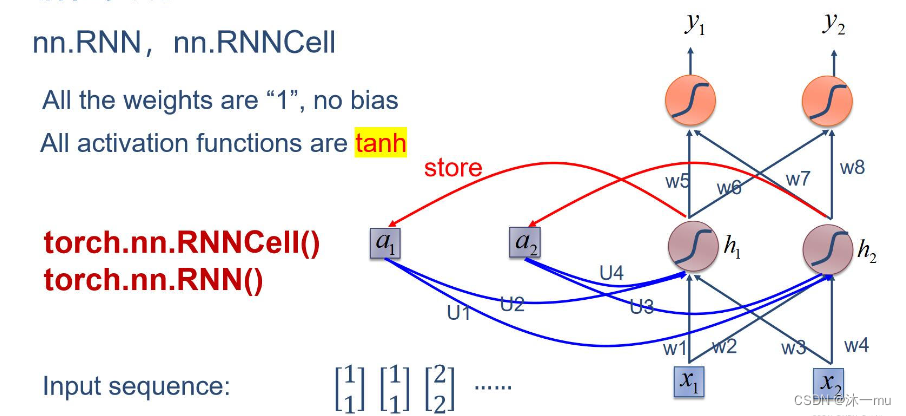
3. 分别使用nn.RNNCell、nn.RNN实现SRN

4. 分析“二进制加法” 源代码（选做）

5. 实现“Character-Level Language Models”源代码（必做）

6. 分析“序列到序列”源代码（选做）

7. “编码器-解码器”的简单实现（必做）

总结：

Ref：

1. 使用Numpy实现SRN

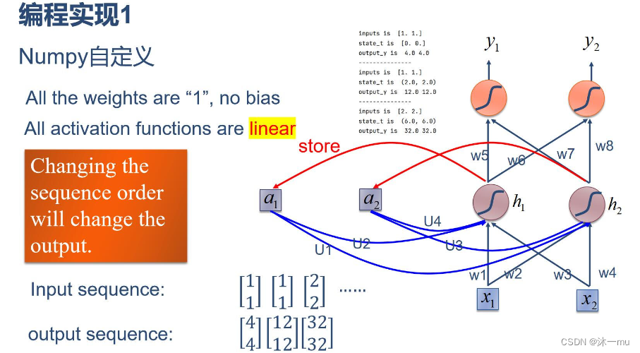
import numpy as npinputs = np.array([[1., 1.],[1., 1.],[2., 2.]])  # 初始化输入序列
print('inputs is ', inputs)state_t = np.zeros(2, )  # 初始化存储器
print('state_t is ', state_t)w1, w2, w3, w4, w5, w6, w7, w8 = 1., 1., 1., 1., 1., 1., 1., 1.
U1, U2, U3, U4 = 1., 1., 1., 1.
print('--------------------------------------')
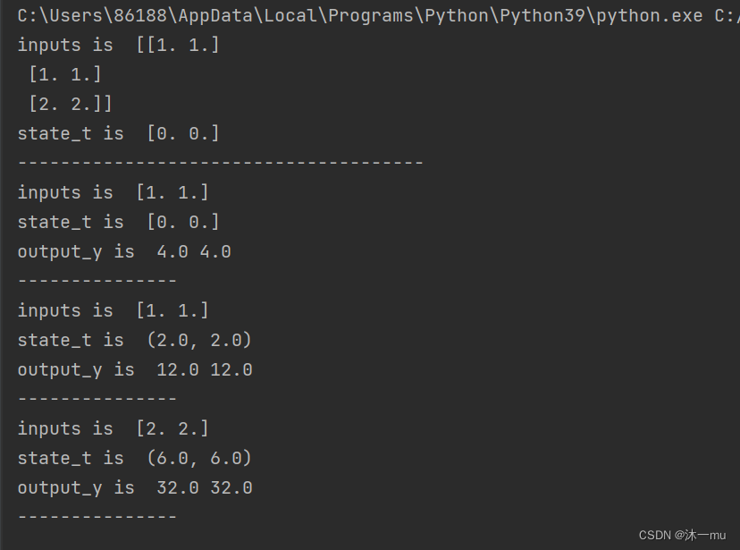
for input_t in inputs:print('inputs is ', input_t)print('state_t is ', state_t)in_h1 = np.dot([w1, w3], input_t) + np.dot([U2, U4], state_t)in_h2 = np.dot([w2, w4], input_t) + np.dot([U1, U3], state_t)state_t = in_h1, in_h2output_y1 = np.dot([w5, w7], [in_h1, in_h2])output_y2 = np.dot([w6, w8], [in_h1, in_h2])print('output_y is ', output_y1, output_y2)print('---------------')

执行结果：

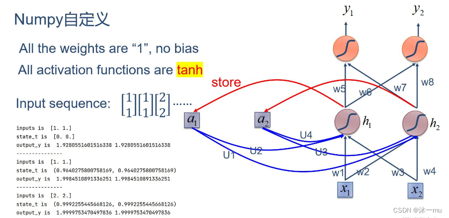
2. 在1的基础上，增加激活函数tanh

import numpy as npinputs = np.array([[1., 1.],[1., 1.],[2., 2.]])  # 初始化输入序列
print('inputs is ', inputs)state_t = np.zeros(2, )  # 初始化存储器
print('state_t is ', state_t)w1, w2, w3, w4, w5, w6, w7, w8 = 1., 1., 1., 1., 1., 1., 1., 1.
U1, U2, U3, U4 = 1., 1., 1., 1.
print('--------------------------------------')
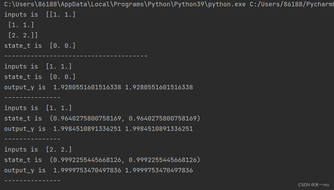
for input_t in inputs:print('inputs is ', input_t)print('state_t is ', state_t)in_h1 = np.tanh(np.dot([w1, w3], input_t) + np.dot([U2, U4], state_t))in_h2 = np.tanh(np.dot([w2, w4], input_t) + np.dot([U1, U3], state_t))state_t = in_h1, in_h2output_y1 = np.dot([w5, w7], [in_h1, in_h2])output_y2 = np.dot([w6, w8], [in_h1, in_h2])print('output_y is ', output_y1, output_y2)print('---------------')

执行结果：

3. 分别使用nn.RNNCell、nn.RNN实现SRN

nn.RNNCell实现SRN

import torchbatch_size = 1
seq_len = 3  # 序列长度
input_size = 2  # 输入序列维度
hidden_size = 2  # 隐藏层维度
output_size = 2  # 输出层维度# RNNCell
cell = torch.nn.RNNCell(input_size=input_size, hidden_size=hidden_size)
# 初始化参数 https://zhuanlan.zhihu.com/p/342012463
for name, param in cell.named_parameters():if name.startswith("weight"):torch.nn.init.ones_(param)else:torch.nn.init.zeros_(param)
# 线性层
liner = torch.nn.Linear(hidden_size, output_size)
liner.weight.data = torch.Tensor([[1, 1], [1, 1]])
liner.bias.data = torch.Tensor([0.0])seq = torch.Tensor([[[1, 1]],[[1, 1]],[[2, 2]]])
hidden = torch.zeros(batch_size, hidden_size)
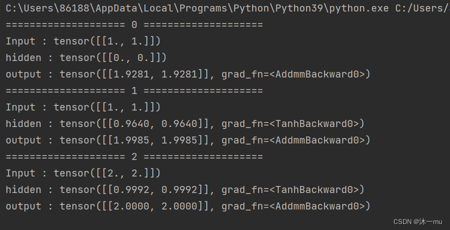
output = torch.zeros(batch_size, output_size)for idx, input in enumerate(seq):print('=' * 20, idx, '=' * 20)print('Input :', input)print('hidden :', hidden)hidden = cell(input, hidden)output = liner(hidden)print('output :', output)

执行结果：

torch.nn.RNN 实现SRN

import torchbatch_size = 1
seq_len = 3
input_size = 2
hidden_size = 2
num_layers = 1
output_size = 2cell = torch.nn.RNN(input_size=input_size, hidden_size=hidden_size, num_layers=num_layers)
for name, param in cell.named_parameters():  # 初始化参数if name.startswith("weight"):torch.nn.init.ones_(param)else:torch.nn.init.zeros_(param)# 线性层
liner = torch.nn.Linear(hidden_size, output_size)
liner.weight.data = torch.Tensor([[1, 1], [1, 1]])
liner.bias.data = torch.Tensor([0.0])inputs = torch.Tensor([[[1, 1]],[[1, 1]],[[2, 2]]])
hidden = torch.zeros(num_layers, batch_size, hidden_size)
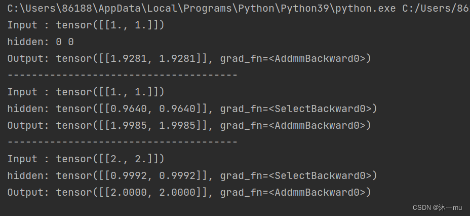
out, hidden = cell(inputs, hidden)print('Input :', inputs[0])
print('hidden:', 0, 0)
print('Output:', liner(out[0]))
print('--------------------------------------')
print('Input :', inputs[1])
print('hidden:', out[0])
print('Output:', liner(out[1]))
print('--------------------------------------')
print('Input :', inputs[2])
print('hidden:', out[1])
print('Output:', liner(out[2]))

执行结果：

4. 分析“二进制加法” 源代码（选做）

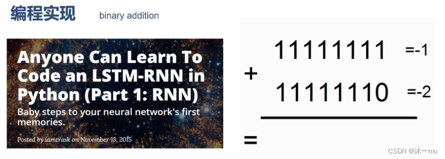
链接：Anyone Can Learn To Code an LSTM-RNN in Python (Part 1: RNN) - i am trask

import copy, numpy as npnp.random.seed(0)#定义sigmoid函数
def sigmoid(x):output = 1 / (1 + np.exp(-x))return output#定义sigmoid导数
def sigmoid_output_to_derivative(output):return output * (1 - output)#训练数据的产生
int2binary = {}
binary_dim = 8 #定义二进制位的长度largest_number = pow(2, binary_dim)#定义数据的最大值
binary = np.unpackbits(np.array([range(largest_number)], dtype=np.uint8).T, axis=1)#函数产生包装所有符合的二进制序列
for i in range(largest_number):#遍历从0-256的值int2binary[i] = binary[i]#对于每个整型值赋值二进制序列
print(int2binary)
# 产生输入变量
alpha = 0.1         #设置更新速度（学习率）
input_dim = 2       #输入维度大小
hidden_dim = 16     #隐藏层维度大小
output_dim = 1      #输出维度大小# 随机产生网络权重
synapse_0 = 2 * np.random.random((input_dim, hidden_dim)) - 1
synapse_1 = 2 * np.random.random((hidden_dim, output_dim)) - 1
synapse_h = 2 * np.random.random((hidden_dim, hidden_dim)) - 1#梯度初始值设置为0
synapse_0_update = np.zeros_like(synapse_0)
synapse_1_update = np.zeros_like(synapse_1)
synapse_h_update = np.zeros_like(synapse_h)#训练逻辑
for j in range(10000):# 产生一个简单的加法问题a_int = np.random.randint(largest_number / 2)  # 产生一个加法操作数a = int2binary[a_int]   # 找到二进制序列编码b_int = np.random.randint(largest_number / 2)  # 产生另一个加法操作数b = int2binary[b_int]   # 找到二进制序列编码# 计算正确值（标签值）c_int = a_int + b_intc = int2binary[c_int]   # 得到正确的结果序列# 设置存储器，存储中间值（记忆功能）d = np.zeros_like(c)overallError = 0        #设置误差layer_2_deltas = list()layer_1_values = list()layer_1_values.append(np.zeros(hidden_dim))# moving along the positions in the binary encodingfor position in range(binary_dim):# 产生输入和输出X = np.array([[a[binary_dim - position - 1], b[binary_dim - position - 1]]])y = np.array([[c[binary_dim - position - 1]]]).T# 隐藏层计算layer_1 = sigmoid(np.dot(X, synapse_0) + np.dot(layer_1_values[-1], synapse_h))# 输出层layer_2 = sigmoid(np.dot(layer_1, synapse_1))# 计算差别layer_2_error = y - layer_2#计算每个梯度layer_2_deltas.append((layer_2_error) * sigmoid_output_to_derivative(layer_2))#计算所有损失overallError += np.abs(layer_2_error[0])# 编码记忆的中间值d[binary_dim - position - 1] = np.round(layer_2[0][0])# 拷贝副本layer_1_values.append(copy.deepcopy(layer_1))future_layer_1_delta = np.zeros(hidden_dim)for position in range(binary_dim):X = np.array([[a[position], b[position]]])layer_1 = layer_1_values[-position - 1]prev_layer_1 = layer_1_values[-position - 2]# 输出层误差layer_2_delta = layer_2_deltas[-position - 1]# 隐藏层误差layer_1_delta = (future_layer_1_delta.dot(synapse_h.T) + layer_2_delta.dot(synapse_1.T)) * sigmoid_output_to_derivative(layer_1)# 计算梯度synapse_1_update += np.atleast_2d(layer_1).T.dot(layer_2_delta)synapse_h_update += np.atleast_2d(prev_layer_1).T.dot(layer_1_delta)synapse_0_update += X.T.dot(layer_1_delta)future_layer_1_delta = layer_1_delta#梯度下降synapse_0 += synapse_0_update * alphasynapse_1 += synapse_1_update * alphasynapse_h += synapse_h_update * alpha#重新初始化synapse_0_update *= 0synapse_1_update *= 0synapse_h_update *= 0# 打印训练过程if (j % 1000 == 0):print("Error:" + str(overallError))print("Pred:" + str(d))print("True:" + str(c))out = 0for index, x in enumerate(reversed(d)):out += x * pow(2, index)print(str(a_int) + " + " + str(b_int) + " = " + str(out))print("------------")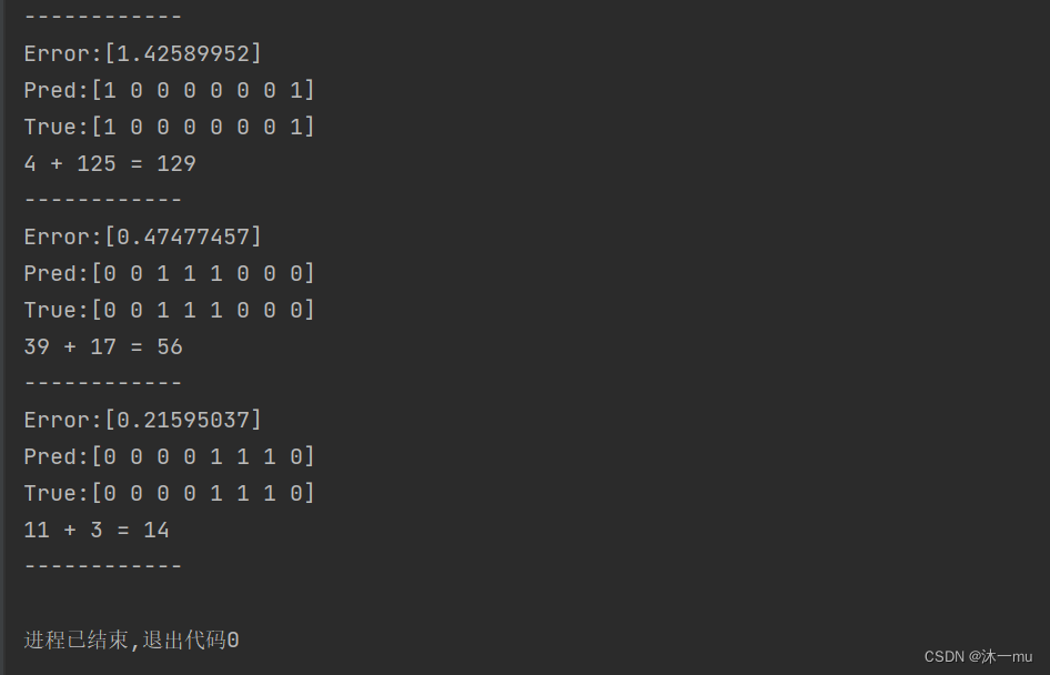

源代码上的注释都很清晰，首先sigmoid和sigmoid导数函数，初始化8位二进制序列的编码，0-256对应其二进制数紧接着随机产生网络权重，设置随机种子保证每次产生的权重相同，d是存储器，
每次训练我们在0-128中随机产生两个数，找到对应的8位二进制序列，进行数据输入。开始训练，每1000次查看一次中间结果，产生的结果和正确的结果进行误差计算，从而更新随机网络权重的参数，再次训练再更新，直至训练结束。

5. 实现“Character-Level Language Models”源代码（必做）

链接：The Unreasonable Effectiveness of Recurrent Neural Networks

import numpy as np
import random
#utils.py中定义了本次实验所需要的辅助函数
#包括朴素RNN的前向/反向传播  和我们在上一个实验中实现的差不多
from utils import *
data = open('D:/dinos.txt', 'r').read() #读取dinos.txt中的所有恐龙名字 read()逐字符读取 返回一个字符串
data= data.lower()#把所有名字转为小写
chars = list(set(data))#得到字符列表并去重
print(chars)  #'a'-'z' '\n'  27个字符
data_size, vocab_size = len(data), len(chars)
print('There are %d total characters and %d unique characters in your data.' % (data_size, vocab_size))
char_to_ix = { ch:i for i,ch in enumerate(sorted(chars)) }
ix_to_char = { i:ch for i,ch in enumerate(sorted(chars)) }
print(ix_to_char)def softmax(x):''''softmax激活函数'''e_x = np.exp(x - np.max(x))  # 首先对输入做一个平移 减去最大值 使其最大值为0 再取exp 避免指数爆炸return e_x / e_x.sum(axis=0)def smooth(loss, cur_loss):return loss * 0.999 + cur_loss * 0.001def print_sample(sample_ix, ix_to_char):'''得到采样的索引对应的字符sample_ix:采样字符的索引ix_to_char:索引到字符的映射字典'''txt = ''.join(ix_to_char[ix] for ix in sample_ix)  # 连接成字符串txt = txt[0].upper() + txt[1:]  # 首字母大写print('%s' % (txt,), end='')def get_initial_loss(vocab_size, seq_length):return -np.log(1.0 / vocab_size) * seq_lengthdef initialize_parameters(n_a, n_x, n_y):"""用小随机数初始化模型参数Returns:parameters -- Python字典包含:Wax -- 与输入相乘的权重矩阵, 维度 (n_a, n_x)Waa -- 与之前隐藏状态相乘的权重矩阵, 维度 (n_a, n_a)Wya -- 与当前隐藏状态相乘用于产生输出的权重矩阵, 维度(n_y,n_a)ba --  计算当前隐藏状态的偏置参数  维度 (n_a, 1)by --  计算当前输出的偏置参数  维度 (n_y, 1)"""np.random.seed(1)Wax = np.random.randn(n_a, n_x) * 0.01Waa = np.random.randn(n_a, n_a) * 0.01Wya = np.random.randn(n_y, n_a) * 0.01b = np.zeros((n_a, 1))by = np.zeros((n_y, 1))parameters = {"Wax": Wax, "Waa": Waa, "Wya": Wya, "b": b, "by": by}return parameters
### GRADED FUNCTION: clipdef clip(gradients, maxValue):'''把每个梯度值剪切到 minimum 和 maximum之间.Arguments:gradients -- Python梯度字典 包含 "dWaa", "dWax", "dWya", "db", "dby"maxValue -- 每个大于maxValue或小于-maxValue的梯度值 被设置为该值Returns:gradients -- Python梯度字典 包含剪切后的切度'''# 取出梯度字典中存储的梯度dWaa, dWax, dWya, db, dby = gradients['dWaa'], gradients['dWax'], gradients['dWya'], gradients['db'], gradients['dby']# 对每个梯度[dWax, dWaa, dWya, db, dby]进行剪切for gradient in [dWax, dWaa, dWya, db, dby]:# gradient[gradient>maxValue] = maxValue# gradient[gradient<-maxValue] = -maxValuenp.clip(gradient, -maxValue, maxValue, out=gradient)gradients = {"dWaa": dWaa, "dWax": dWax, "dWya": dWya, "db": db, "dby": dby}return gradients# GRADED FUNCTION: sampledef sample(parameters, char_to_ix, seed):"""根据朴素RNN输出的概率分布对字符序列进行采样Arguments:parameters --Python字典 包含模型参数 Waa, Wax, Wya, by, and b.char_to_ix -- Python字典 把每个字符映射为索引seed -- .Returns:indices -- 包含采样字符索引的列表."""# 得到模型参数 和相关维度信息Waa, Wax, Wya, by, b = parameters['Waa'], parameters['Wax'], parameters['Wya'], parameters['by'], parameters['b']vocab_size = by.shape[0]  # 字典大小  输出单元的数量n_a = Waa.shape[1]  # 隐藏单元数量# Step 1: 创建第一个时间步骤上输入的初始向量 初始化序列生成x = np.zeros((vocab_size, 1))# Step 1': 初始化a_preva_prev = np.zeros((n_a, 1))# 保存生成字符index的列表indices = []# 检测换行符, 初始化为 -1idx = -1# 在每个时间步骤上进行循环.在每个时间步骤输出的概率分布上采样一个字符# 把采样字典的index添加到indices中. 如果达到50个字符就停止 (说明模型训练有点问题)#  用于终止无限循环   模型如果训练的不错的话  在遇到换行符之前不会达到50个字符counter = 0newline_character = char_to_ix['\n']  # 换行符索引while (idx != newline_character and counter != 50):  # 如果生成的字符不是换行符且循环次数小于50  就继续# Step 2: 对x进行前向传播   公式(1), (2) and (3)a = np.tanh(Wax.dot(x) + Waa.dot(a_prev) + b)  # (n_a,1)z = Wya.dot(a) + by  # (n_y,1)y = softmax(z)  # (n_y,1)np.random.seed(counter + seed)# Step 3:从输出的概率分布y中 采样一个字典中的字符索引idx = np.random.choice(range(vocab_size), p=y.ravel())indices.append(idx)# Step 4: 根据采样的索引 得到对应字符的one-hot形式 重写输入xx = np.zeros((vocab_size, 1))x[idx] = 1# 更新a_preva_prev = aseed += 1counter += 1if (counter == 50):indices.append(char_to_ix['\n'])return indicesdef rnn_step_forward(parameters, a_prev, x):'''朴素RNN单元的前行传播'''# 从参数字典中取出参数Waa, Wax, Wya, by, b = parameters['Waa'], parameters['Wax'], parameters['Wya'], parameters['by'], parameters['b']# 计算当前时间步骤上的隐藏状态a_next = np.tanh(np.dot(Wax, x) + np.dot(Waa, a_prev) + b)# 计算当前时间步骤上的预测输出  通过一个输出层(使用softmax激活函数，多分类 ，类别数为字典大小)p_t = softmax(np.dot(Wya, a_next) + by)return a_next, p_tdef rnn_step_backward(dy, gradients, parameters, x, a, a_prev):'''朴素RNN单元的反向传播'''gradients['dWya'] += np.dot(dy, a.T)gradients['dby'] += dyda = np.dot(parameters['Wya'].T, dy) + gradients['da_next']  # backprop into hdaraw = (1 - a * a) * da  # backprop through tanh nonlinearitygradients['db'] += darawgradients['dWax'] += np.dot(daraw, x.T)gradients['dWaa'] += np.dot(daraw, a_prev.T)gradients['da_next'] = np.dot(parameters['Waa'].T, daraw)return gradientsdef update_parameters(parameters, gradients, lr):'''使用随机梯度下降法更新模型参数parameters：模型参数字典gradients：对模型参数计算的梯度lr：学习率'''parameters['Wax'] += -lr * gradients['dWax']parameters['Waa'] += -lr * gradients['dWaa']parameters['Wya'] += -lr * gradients['dWya']parameters['b'] += -lr * gradients['db']parameters['by'] += -lr * gradients['dby']return parametersdef rnn_forward(X, Y, a0, parameters, vocab_size=27):'''朴素RNN的前行传播和上一个实验实验的RNN有所不同，之前我们一次处理m个样本/序列 要求m个序列有相同的长度本次实验的RNN，一次只处理一个样本/序列(名字单词) 所以不用统一长度。X -- 整数列表，每个数字代表一个字符的索引。 X是一个训练样本 代表一个单词Y -- 整数列表，每个数字代表一个字符的索引。 Y是一个训练样本对应的真实标签 为X中的索引左移一位'''# Initialize x, a and y_hat as empty dictionariesx, a, y_hat = {}, {}, {}a[-1] = np.copy(a0)# initialize your loss to 0loss = 0for t in range(len(X)):# 设置x[t]为one-hot向量形式.# 如果 X[t] == None, 设置 x[t]=0向量. 设置第一个时间步骤的输入为0向量x[t] = np.zeros((vocab_size, 1))  # 设置每个时间步骤的输入向量if (X[t] != None):x[t][X[t]] = 1  # one-hot形式 索引位置为1 其余为0# 运行一步RNN前向传播a[t], y_hat[t] = rnn_step_forward(parameters, a[t - 1], x[t])# 得到当前时间步骤的隐藏状态和预测输出# 把预测输出和真实标签结合 计算交叉熵损失loss -= np.log(y_hat[t][Y[t], 0])cache = (y_hat, a, x)return loss, cachedef rnn_backward(X, Y, parameters, cache):'''朴素RNN的反向传播'''# Initialize gradients as an empty dictionarygradients = {}# Retrieve from cache and parameters(y_hat, a, x) = cacheWaa, Wax, Wya, by, b = parameters['Waa'], parameters['Wax'], parameters['Wya'], parameters['by'], parameters['b']# each one should be initialized to zeros of the same dimension as its corresponding parametergradients['dWax'], gradients['dWaa'], gradients['dWya'] = np.zeros_like(Wax), np.zeros_like(Waa), np.zeros_like(Wya)gradients['db'], gradients['dby'] = np.zeros_like(b), np.zeros_like(by)gradients['da_next'] = np.zeros_like(a[0])### START CODE HERE #### Backpropagate through timefor t in reversed(range(len(X))):dy = np.copy(y_hat[t])dy[Y[t]] -= 1gradients = rnn_step_backward(dy, gradients, parameters, x[t], a[t], a[t - 1])### END CODE HERE ###return gradients, a# GRADED FUNCTION: optimizedef optimize(X, Y, a_prev, parameters, learning_rate=0.01):"""执行一步优化过程(随机梯度下降，一次优化使用一个训练训练).Arguments:X -- 整数列表，每个数字代表一个字符的索引。 X是一个训练样本 代表一个单词Y -- 整数列表，每个数字代表一个字符的索引。 Y是一个训练样本对应的真实标签 为X中的索引左移一位a_prev -- 上一个时间步骤产生的隐藏状态parameters -- Python字典包含:Wax -- 与输入相乘的权重矩阵, 维度 (n_a, n_x)Waa -- 与之前隐藏状态相乘的权重矩阵, 维度 (n_a, n_a)Wya -- 与当前隐藏状态相乘用于产生输出的权重矩阵, 维度 (n_y, n_a)ba --  计算当前隐藏状态的偏置参数  维度 (n_a, 1)by --  计算当前输出的偏置参数  维度 (n_y, 1)learning_rate -- 学习率Returns:loss -- loss函数值(交叉熵)gradients -- python dictionary containing:dWax -- Gradients of input-to-hidden weights, of shape (n_a, n_x)dWaa -- Gradients of hidden-to-hidden weights, of shape (n_a, n_a)dWya -- Gradients of hidden-to-output weights, of shape (n_y, n_a)db -- Gradients of bias vector, of shape (n_a, 1)dby -- Gradients of output bias vector, of shape (n_y, 1)a[len(X)-1] -- 最后一个隐藏状态 (n_a, 1)"""# 通过时间前向传播loss, cache = rnn_forward(X, Y, a_prev, parameters, vocab_size=27)# 通过时间的反向传播gradients, a = rnn_backward(X, Y, parameters, cache)# 梯度剪切 -5 (min)  5 (max)gradients = clip(gradients, maxValue=5)# 更新参数parameters = update_parameters(parameters, gradients, lr=learning_rate)return loss, gradients, a[len(X) - 1]# GRADED FUNCTION: modeldef model(data, ix_to_char, char_to_ix, num_iterations=35000, n_a=50, dino_names=7, vocab_size=27):"""训练模型生成恐龙名字.Arguments:data -- 文本语料(恐龙名字数据集)ix_to_char -- 从索引到字符的映射字典char_to_ix -- 从字符到索引的映射字典num_iterations -- 随机梯度下降的迭代次数  每次使用一个训练样本(一个名字)n_a -- RNN单元中的隐藏单元数dino_names -- 采样的恐龙名字数量vocab_size -- 字典的大小  文本语料中不同的字符数Returns:parameters --  训练好的参数"""# 输入特征向量x的维度n_x, 输出预测概率向量的维度n_y  2者都为字典大小n_x, n_y = vocab_size, vocab_size# 初始化参数parameters = initialize_parameters(n_a, n_x, n_y)# 初始化loss (this is required because we want to smooth our loss, don't worry about it)loss = get_initial_loss(vocab_size, dino_names)# 得到所有恐龙名字的列表 (所有训练样本).with open("D:/dinos.txt") as f:examples = f.readlines()  # 读取所有行 每行是一个名字 作为列表的一个元素examples = [x.lower().strip() for x in examples]  # 转换小写 去掉换行符# 随机打乱所有恐龙名字 所有训练样本np.random.seed(0)np.random.shuffle(examples)# 初始化隐藏状态为0a_prev = np.zeros((n_a, 1))# 优化循环for j in range(num_iterations):# 得到一个训练样本 (X,Y)index = j % len(examples)  # 得到随机打乱后的一个名字的索引X = [None] + [char_to_ix[ch] for ch in examples[index]]  # 把名字中的每个字符转为对应的索引 第一个字符为None翻译为0向量Y = X[1:] + [char_to_ix['\n']]# 随机梯度下降 执行一次优化: Forward-prop -> Backward-prop -> Clip -> Update parameters# 学习率 0.01curr_loss, gradients, a_prev = optimize(X, Y, a_prev, parameters, learning_rate=0.01)# 使用延迟技巧保持loss平稳. 加速训练loss = smooth(loss, curr_loss)# 每2000次随机梯度下降迭代, 通过sample()生成'n'个字符(1个名字)  来检查模型是否训练正确if j % 2000 == 0:print('Iteration: %d, Loss: %f' % (j, loss) + '\n')seed = 0for name in range(dino_names):  # 生成名字的数量# 得到采样字符的索引sampled_indices = sample(parameters, char_to_ix, seed)# 得到索引对应的字符 生成一个名字print_sample(sampled_indices, ix_to_char)seed += 1  # To get the same result for grading purposed, increment the seed by one.print('\n')return parameters
parameters = model(data, ix_to_char, char_to_ix) #训练模型

翻译：the sequence regime of operation is much more powerful compared to fixed networks that are doomed from the get-go by a fixed number of computational steps, and hence also much more appealing for those of us who aspire to build more intelligent systems. Moreover, as we’ll see in a bit, RNNs combine the input vector with their state vector with a fixed (but learned) function to produce a new state vector. This can in programming terms be interpreted as running a fixed program with certain inputs and some internal variables. Viewed this way, RNNs essentially describe programs. In fact, it is known that RNNs are Turing-Complete in the sense that they can to simulate arbitrary programs (with proper weights).

与固定网络相比，操作的序列机制要强大得多，固定网络从一开始就注定要通过固定数量的计算步骤来失败，因此对于我们这些渴望构建更智能系统的人来说也更具吸引力。此外，正如我们稍后将看到的，RNN 将输入向量与其状态向量与固定（但已学习）函数相结合，以产生新的状态向量。这在编程术语中可以解释为运行具有某些输入和一些内部变量的固定程序。从这个角度来看，RNN本质上描述了程序。事实上，众所周知，RNN 是图灵完备的，因为它们可以模拟任意程序（具有适当的权重）。

Okay, so we have an idea about what RNNs are, why they are super exciting, and how they work. We’ll now ground this in a fun application: We’ll train RNN character-level language models. That is, we’ll give the RNN a huge chunk of text and ask it to model the probability distribution of the next character in the sequence given a sequence of previous characters. This will then allow us to generate new text one character at a time.

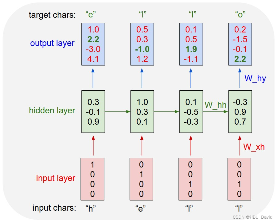
As a working example, suppose we only had a vocabulary of four possible letters “helo”, and wanted to train an RNN on the training sequence “hello”. This training sequence is in fact a source of 4 separate training examples: 1. The probability of “e” should be likely given the context of “h”, 2. “l” should be likely in the context of “he”, 3. “l” should also be likely given the context of “hel”, and finally 4. “o” should be likely given the context of “hell”.

Concretely, we will encode each character into a vector using 1-of-k encoding (i.e. all zero except for a single one at the index of the character in the vocabulary), and feed them into the RNN one at a time with the function. We will then observe a sequence of 4-dimensional output vectors (one dimension per character), which we interpret as the confidence the RNN currently assigns to each character coming next in the sequence. Here’s a diagram:

好的，所以我们有一个关于RNN是什么，为什么它们超级令人兴奋的，以及它们是如何工作的。现在，我们将在一个有趣的应用程序中进行验证：我们将训练 RNN 字符级语言模型。也就是说，我们将给 RNN 一大块文本，并要求它对给定先前字符序列的序列中下一个字符的概率分布进行建模。然后，这将允许我们一次生成一个字符的新文本。

作为一个工作示例，假设我们只有四个可能的字母“helo”的词汇表，并且想在训练序列“hello”上训练一个RNN。这个训练序列实际上是 4 个独立训练示例的来源：1. 给定 “h” 上下文时，“e”的概率应该可能，2. “l”应该在“he”的上下文中出现，3. “l”也应该在给定“hel”的上下文中，最后是 4。“o”应该可能被赋予“地狱”的上下文。

具体来说，我们将使用 1-of-k 编码将每个字符编码到一个向量中（即除了词汇表中字符索引处的单个字符之外的所有字符均为零），并使用函数一次将它们馈送到 RNN 中。然后，我们将观察一个 4 维输出向量序列（每个字符一个维度），我们将其解释为 RNN 当前分配给序列中下一个字符的置信度。下图如下：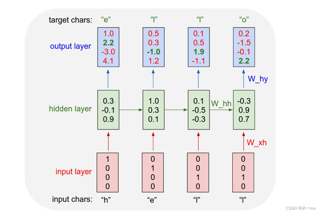

6. 分析“序列到序列”源代码（选做）

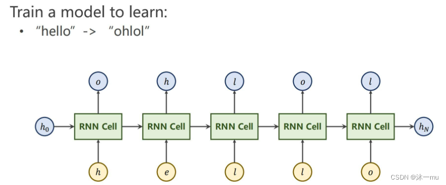
h0相当于初始隐状态输入，h是正常的输入，1、2、3、4分别是不同的隐状态进入到下一个RNN Cell中去，由上一个的隐状态向量和当前输入确定当前输出和隐状态向量输出，从而将“hello”翻译成了"ohlol".

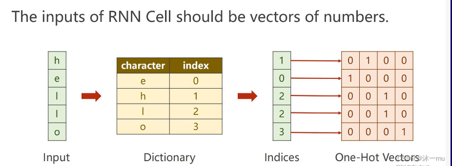
按照这个字典对“hello进行编码”（这里是独热编码）得到的码片序列为：0100 1000 0010 0010 0001从而喂入数据进行运算，喂入之后，通过初始化隐状态向量和当前输入做隐状态向量的更新和当前的一个输出，再进行解码器按照字典对照表解码，从而输出第一个字母，依次类推，从而得到输出序列，这里我没有找到代码，所以没有做具体分析，只能按照图来分析其过程。

7. “编码器-解码器”的简单实现（必做）

# Model
class Seq2Seq(nn.Module):def __init__(self):super(Seq2Seq, self).__init__()self.encoder = nn.RNN(input_size=n_class, hidden_size=n_hidden, dropout=0.5) # encoderself.decoder = nn.RNN(input_size=n_class, hidden_size=n_hidden, dropout=0.5) # decoderself.fc = nn.Linear(n_hidden, n_class)def forward(self, enc_input, enc_hidden, dec_input):# enc_input(=input_batch): [batch_size, n_step+1, n_class]# dec_inpu(=output_batch): [batch_size, n_step+1, n_class]enc_input = enc_input.transpose(0, 1) # enc_input: [n_step+1, batch_size, n_class]dec_input = dec_input.transpose(0, 1) # dec_input: [n_step+1, batch_size, n_class]# h_t : [num_layers(=1) * num_directions(=1), batch_size, n_hidden]_, h_t = self.encoder(enc_input, enc_hidden)# outputs : [n_step+1, batch_size, num_directions(=1) * n_hidden(=128)]outputs, _ = self.decoder(dec_input, h_t)model = self.fc(outputs) # model : [n_step+1, batch_size, n_class]return modelmodel = Seq2Seq().to(device)
criterion = nn.CrossEntropyLoss().to(device)
optimizer = torch.optim.Adam(model.parameters(), lr=0.001)

# code by Tae Hwan Jung(Jeff Jung) @graykode, modify by wmathor
import torch
import numpy as np
import torch.nn as nn
import torch.utils.data as Datadevice = torch.device('cuda' if torch.cuda.is_available() else 'cpu')
# S: Symbol that shows starting of decoding input
# E: Symbol that shows starting of decoding output
# ?: Symbol that will fill in blank sequence if current batch data size is short than n_stepletter = [c for c in 'SE?abcdefghijklmnopqrstuvwxyz']
letter2idx = {n: i for i, n in enumerate(letter)}seq_data = [['man', 'women'], ['black', 'white'], ['king', 'queen'], ['girl', 'boy'], ['up', 'down'], ['high', 'low']]# Seq2Seq Parameter
n_step = max([max(len(i), len(j)) for i, j in seq_data]) # max_len(=5)
n_hidden = 128
n_class = len(letter2idx) # classfication problem
batch_size = 3def make_data(seq_data):enc_input_all, dec_input_all, dec_output_all = [], [], []for seq in seq_data:for i in range(2):seq[i] = seq[i] + '?' * (n_step - len(seq[i])) # 'man??', 'women'enc_input = [letter2idx[n] for n in (seq[0] + 'E')] # ['m', 'a', 'n', '?', '?', 'E']dec_input = [letter2idx[n] for n in ('S' + seq[1])] # ['S', 'w', 'o', 'm', 'e', 'n']dec_output = [letter2idx[n] for n in (seq[1] + 'E')] # ['w', 'o', 'm', 'e', 'n', 'E']enc_input_all.append(np.eye(n_class)[enc_input])dec_input_all.append(np.eye(n_class)[dec_input])dec_output_all.append(dec_output) # not one-hot# make tensorreturn torch.Tensor(enc_input_all), torch.Tensor(dec_input_all), torch.LongTensor(dec_output_all)'''
enc_input_all: [6, n_step+1 (because of 'E'), n_class]
dec_input_all: [6, n_step+1 (because of 'S'), n_class]
dec_output_all: [6, n_step+1 (because of 'E')]
'''
enc_input_all, dec_input_all, dec_output_all = make_data(seq_data)class TranslateDataSet(Data.Dataset):def __init__(self, enc_input_all, dec_input_all, dec_output_all):self.enc_input_all = enc_input_allself.dec_input_all = dec_input_allself.dec_output_all = dec_output_alldef __len__(self): # return dataset sizereturn len(self.enc_input_all)def __getitem__(self, idx):return self.enc_input_all[idx], self.dec_input_all[idx], self.dec_output_all[idx]loader = Data.DataLoader(TranslateDataSet(enc_input_all, dec_input_all, dec_output_all), batch_size, True)# Model
class Seq2Seq(nn.Module):def __init__(self):super(Seq2Seq, self).__init__()self.encoder = nn.RNN(input_size=n_class, hidden_size=n_hidden, dropout=0.5) # encoderself.decoder = nn.RNN(input_size=n_class, hidden_size=n_hidden, dropout=0.5) # decoderself.fc = nn.Linear(n_hidden, n_class)def forward(self, enc_input, enc_hidden, dec_input):# enc_input(=input_batch): [batch_size, n_step+1, n_class]# dec_inpu(=output_batch): [batch_size, n_step+1, n_class]enc_input = enc_input.transpose(0, 1) # enc_input: [n_step+1, batch_size, n_class]dec_input = dec_input.transpose(0, 1) # dec_input: [n_step+1, batch_size, n_class]# h_t : [num_layers(=1) * num_directions(=1), batch_size, n_hidden]_, h_t = self.encoder(enc_input, enc_hidden)# outputs : [n_step+1, batch_size, num_directions(=1) * n_hidden(=128)]outputs, _ = self.decoder(dec_input, h_t)model = self.fc(outputs) # model : [n_step+1, batch_size, n_class]return modelmodel = Seq2Seq().to(device)
criterion = nn.CrossEntropyLoss().to(device)
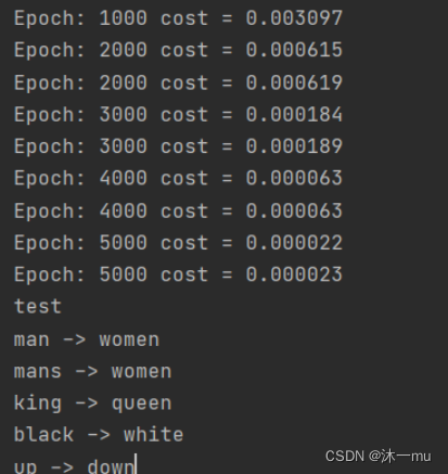
optimizer = torch.optim.Adam(model.parameters(), lr=0.001)for epoch in range(5000):for enc_input_batch, dec_input_batch, dec_output_batch in loader:# make hidden shape [num_layers * num_directions, batch_size, n_hidden]h_0 = torch.zeros(1, batch_size, n_hidden).to(device)(enc_input_batch, dec_intput_batch, dec_output_batch) = (enc_input_batch.to(device), dec_input_batch.to(device), dec_output_batch.to(device))# enc_input_batch : [batch_size, n_step+1, n_class]# dec_intput_batch : [batch_size, n_step+1, n_class]# dec_output_batch : [batch_size, n_step+1], not one-hotpred = model(enc_input_batch, h_0, dec_intput_batch)# pred : [n_step+1, batch_size, n_class]pred = pred.transpose(0, 1) # [batch_size, n_step+1(=6), n_class]loss = 0for i in range(len(dec_output_batch)):# pred[i] : [n_step+1, n_class]# dec_output_batch[i] : [n_step+1]loss += criterion(pred[i], dec_output_batch[i])if (epoch + 1) % 1000 == 0:print('Epoch:', '%04d' % (epoch + 1), 'cost =', '{:.6f}'.format(loss))optimizer.zero_grad()loss.backward()optimizer.step()# Test
def translate(word):enc_input, dec_input, _ = make_data([[word, '?' * n_step]])enc_input, dec_input = enc_input.to(device), dec_input.to(device)# make hidden shape [num_layers * num_directions, batch_size, n_hidden]hidden = torch.zeros(1, 1, n_hidden).to(device)output = model(enc_input, hidden, dec_input)# output : [n_step+1, batch_size, n_class]predict = output.data.max(2, keepdim=True)[1] # select n_class dimensiondecoded = [letter[i] for i in predict]translated = ''.join(decoded[:decoded.index('E')])return translated.replace('?', '')print('test')
print('man ->', translate('man'))
print('mans ->', translate('mans'))
print('king ->', translate('king'))
print('black ->', translate('black'))
print('up ->', translate('up'))

总结：

RNN（Recurrent Neural Network）是一类用于处理序列数据的神经网络。首先我们要明确什么是序列数据，摘取百度百科词条：时间序列数据是指在不同时间点上收集到的数据，这类数据反映了某一事物、现象等随时间的变化状态或程度。这是时间序列数据的定义，当然这里也可以不是时间，比如文字序列，但总归序列数据有一个特点——后面的数据跟前面的数据有关系。

RNN是神经网络的一种，类似的还有深度神经网络DNN，卷积神经网络CNN，生成对抗网络GAN，等等。RNN对具有序列特性的数据非常有效，它能挖掘数据中的时序信息以及语义信息，利用了RNN的这种能力，使深度学习模型在解决语音识别、语言模型、机器翻译以及时序分析等NLP领域的问题时有所突破。

举几个具有序列特性的例子：

拿人类的某句话来说，也就是人类的自然语言，是不是符合某个逻辑或规则的字词拼凑排列起来的，这就是符合序列特性。
语音，我们发出的声音，每一帧每一帧的衔接起来，才凑成了我们听到的话，这也具有序列特性。
股票，随着时间的推移，会产生具有顺序的一系列数字，这些数字也是具有序列特性。
这次也翻译了一些英文文献，虽然比较难懂，但深入思考的话还是能学到很多东西。