目标检测2——借Detectron2源码理解Anchors与RPN

文章目录

- 1.Regionn Proposal Network背景
- 2.Regionn Proposal Network的结构
- 3.Anchors
- 4.Regionn Proposal Network的训练
- 参考资料

欢迎访问个人网络日志🌹🌹知行空间🌹🌹

1.Regionn Proposal Network背景

RPN，Region Proposal Network是中科大与微软亚洲研究院联合培养博士,原Momenta研发总监任少卿与何凯明，Ross Girshick共同发表的论文Faster R-CNN中提出的一个网络结构，用于目标检测，RPN论文最早发表于2015年06月04号,是在Fast RCNN上的改进，与其一起提出的Translation-Invariant Anchors极大的提高的检测的性呢和准确度。Faster R-CNN使用RPN和anchors替代RCNN和Fast RCNN中的selective search方法，Faster R-CNN将检测问题分成了特征提取backcbone的训练和RPN候选框生成网络的训练，因此是Two Stage检测框架。RPN用于生成Proposal Boxes, 以用来输入ROI Pooling和ROI Align，做进一步的类别判断和检测框定位。

因RPN是Faster R-CNN中提出的，先来看下Faster R-CNN的整体结构：
在这里插入图片描述

上图中，可以看到，对于输入的图像，先经过Conv Layers进行特征提取得到feature map,再将feature map一支用于输入RPN结合anchors来生成Proposal Boxes,另一支feature map和RPN生成的Proposal boxes一起输入ROI Pooling,经过全连接层后做检测物体类别的回归和检测框的精细化定位。从上图中可以知道，RPN网络的作用就是输入feature map,输出Proposal Boxes,在进行检测网络整体训练之前，需基于现有的Model先训练RPN网络，使其能够用来生成Proposal Boxes,然后再训练Model,循环3次。

2.Regionn Proposal Network的结构

在这里插入图片描述

如图，这是目前R-CNN衍生出来的检测算法都会使用的RPN Head的网络结构，用来生成Proposal Boxes,并判断其中是否包含物体,输出每个Proposal Boxes的置信度。结合上图，介绍一下rpn网络的结构，RPN网络的输入是backbone提取得到的feature map（NCHW),网络结构中先有一个3x3的卷积，进一步融合特征，然后将卷积结果分别输入到两个分支上。每个分支都包含一个1x1的卷积，只改变输入特征图的通道大小，不改变feature map的宽高。其中一支负责预测anchors偏移量，输出通道数变为num_anchors*box_dims,关于anchors的介绍见下一部分。另一支负责预测每个proposal boxes的置信度，其输出通道数为num_anchors。因总的proposal boxes数里过多，得到置信度和proposal boxes对应的位置后，可据此对proposal boxes进行过滤，正是图中proposals层做的事情，其介绍见图2,这里是以一个feature map进行说明的，对于FPN结构的网络，对不同层级的特征分别进行处理即可。代码实现可以参考detectron2

class StandardRPNHead(nn.Module):def forward(self, features: List[torch.Tensor]):"""Args:features (list[Tensor]): list of feature mapsReturns:list[Tensor]: A list of L elements.Element i is a tensor of shape (N, A, Hi, Wi) representingthe predicted objectness logits for all anchors. A is the number of cell anchors.list[Tensor]: A list of L elements. Element i is a tensor of shape(N, A*box_dim, Hi, Wi) representing the predicted "deltas" used to transform anchorsto proposals."""pred_objectness_logits = []pred_anchor_deltas = []for x in features:t = self.conv(x)pred_objectness_logits.append(self.objectness_logits(t))pred_anchor_deltas.append(self.anchor_deltas(t))return pred_objectness_logits, pred_anchor_deltas

3.Anchors

‵Anchors是Faster RCNN论文中提出的用来更好的回归bounding boxes`的算法。

_C.MODEL.ANCHOR_GENERATOR.SIZES = [[32, 64, 128, 256, 512]]
# Anchor aspect ratios. For each area given in `SIZES`, anchors with different aspect
# ratios are generated by an anchor generator.
# Format: list[list[float]]. ASPECT_RATIOS[i] specifies the list of aspect ratios (H/W)
# to use for IN_FEATURES[i]; len(ASPECT_RATIOS) == len(IN_FEATURES) must be true,
# or len(ASPECT_RATIOS) == 1 is true and aspect ratio list ASPECT_RATIOS[0] is used
# for all IN_FEATURES.
_C.MODEL.ANCHOR_GENERATOR.ASPECT_RATIOS = [[0.5, 1.0, 2.0]]

如上代码中，分别是5种size，3种宽高比的Anchors配置，Anchors的大小是在检测输入图像的尺度上的，通过变换可知对于每个点共有15种不同宽高比和大小的anchors,

在这里插入图片描述

Anchors是作用在feature map上的每个cell中心点的，再根据图像信息和特征提取网络的stride，找到原图上Anchors的对应位置。其应用可以参考faster rcnn论文的一个图，

在这里插入图片描述

使用Anchors时，bounding boxes回归的原理是anchors的中心 $x, y$ 和宽高 $w, h$ 通过平移和缩放可以得到对应的bounding box。给定 $anchor A(A_x, A_y, A_w, A_h)$ 和 $gt G(G_x, G_y,G_w, G_h)$ 可以寻找一种变换F使得 $F(A_x, A_y, A_w, A_h)=G'(G_x', G_y', G_w', G_h')$ ，而 $G\approx G'$ ,变换F可以表示为：

先平移
$\begin{matrix} G_x'=A_w*d_x(A)+A_x \\ G_y'=A_h*d_x(A)+A_y \end{matrix}$
再缩放

$G_w'=A_w exp(d_w(A)) \\ G_h'=A_h exp(d_h(A))$

其中 $d_x(A),d_y(A),d_w(A),d_h(A)$ 四个变换，当anchor与gt box相差很小时，可看成线性变换即Y=WX。

在这里插入图片描述

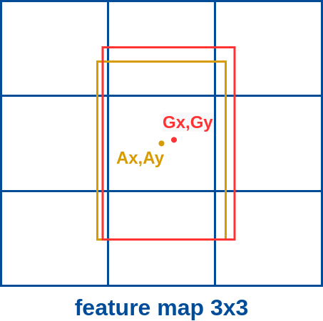
上图种蓝色的网格表示feature map特征图，在其中间一个cell上生成的一个Anchor如图中黄色框所示，其中心 $A_x,A_y$ 取cell的中心对应的原图上的坐标，与当前这个对应IoU最大的ground truth box如图中红色的框，其中心坐标为 $G_x,G_y$ ,可以知道一般情况下Anchor只是大概定位了检测框的位置，还需对其进行少量的平移才能实现准确定位。同样Anchor也只是大概确定了检测框的宽高，还需在宽高方向上进行适量的缩放才能得到准确的检测框。

faster rcnn中的偏移量预测是tx,没有范围限制，容易导致产生超出边界的预测框，在2016年12月25号Joseph Redmon发表的Yolov2中对其进行了修改，改成了在预测相对于featue map cell左上点的偏移量，并做sigmoid，使得偏移量始终在 $0 - 1$ 之间。

对于检测网络训练时，传入A与Ground Truth Boxes之间的变换量 $t_x, t_y, t_\omega,t_h$ ,借此使用L1损失函数回归Y=WX函数即可完成RPN的训练。

4.Regionn Proposal Network的训练

训练RPN网络时，需先将feaure map经过RPN前向推理得到shape=(N, Hi*Wi*A)的pred_objectness_logits scores和shape=(N, Hi*Wi*A, B)的pred_anchor_deltas。然后将shape = [N, H*W*A]的anchors和shape=[N, M, B]的ground truth boxes对应起来，再计算含有物体的positive target anchors和predicted anchors之间的定位损失及positive and negative target anchors和对应predicted anchors之间的分类损失。

训练RPN网络时，比较多的工作花费在了anchor assignment,即实现anchors与ground truth box之间的匹配。faster R-CNN中主要使用的anchor与ground truth box之间的IoU来实现。对于M个anchors和N个round truth boxes，两两之间分别计算IoU,可以得到MxN的IoU_Match矩阵，取每个anchor与N个gt boxes IoU最大的box作为与anchor匹配的Ground Truth Box,如此找到了每个anchor对应的Ground Truth Box。再根据两者之间的IoU，判断其是背景bg还是前景fg即是否有物体，判断方式通常是设者IoU_Threshold_Low和IoU_Threshold_High，IoU大于IoU_Threshold_High的是positive,小于IoU_Threshold_Low的是negative，介于两者之间的忽略。通过这样定义可以知道一个ground truth box可以对应多个anchor。初步判断出positive/negative anchors之后，还需经过超参数每个图像中训练最多使用的anchor box数量和其中positive anchors fraction对anchors再次处理，限制参与训练的anchor box不多于超参数最大数量，见detectron2 rpn.py中的label_and_sample_anchors函数。

def label_and_sample_anchors(self, anchors: List[Boxes], gt_instances: List[Instances]
) -> Tuple[List[torch.Tensor], List[torch.Tensor]]:anchors = Boxes.cat(anchors)gt_boxes = [x.gt_boxes for x in gt_instances]image_sizes = [x.image_size for x in gt_instances]del gt_instancesgt_labels = []matched_gt_boxes = []for image_size_i, gt_boxes_i in zip(image_sizes, gt_boxes):"""image_size_i: (h, w) for the i-th imagegt_boxes_i: ground-truth boxes for i-th image"""match_quality_matrix = retry_if_cuda_oom(pairwise_iou)(gt_boxes_i, anchors)matched_idxs, gt_labels_i = retry_if_cuda_oom(self.anchor_matcher)(match_quality_matrix)# M个anchors与N个ground truth boxes匹配，得到M个anchors分别对应的ground truth box，找到每个anchor的标签gt_labels_i = gt_labels_i.to(device=gt_boxes_i.device)del match_quality_matrixif self.anchor_boundary_thresh >= 0:# Discard anchors that go out of the boundaries of the image# NOTE: This is legacy functionality that is turned off by default in Detectron2anchors_inside_image = anchors.inside_box(image_size_i, self.anchor_boundary_thresh)gt_labels_i[~anchors_inside_image] = -1# A vector of labels (-1, 0, 1) for each anchor# 根据超参数，限制每张图像中参与训练的anchors上限和positive anchor的比例gt_labels_i = self._subsample_labels(gt_labels_i)if len(gt_boxes_i) == 0:# These values won't be used anyway since the anchor is labeled as backgroundmatched_gt_boxes_i = torch.zeros_like(anchors.tensor)else:# TODO wasted indexing computation for ignored boxesmatched_gt_boxes_i = gt_boxes_i[matched_idxs].tensorgt_labels.append(gt_labels_i)  # N,AHWmatched_gt_boxes.append(matched_gt_boxes_i)return gt_labels, matched_gt_boxes

损失函数

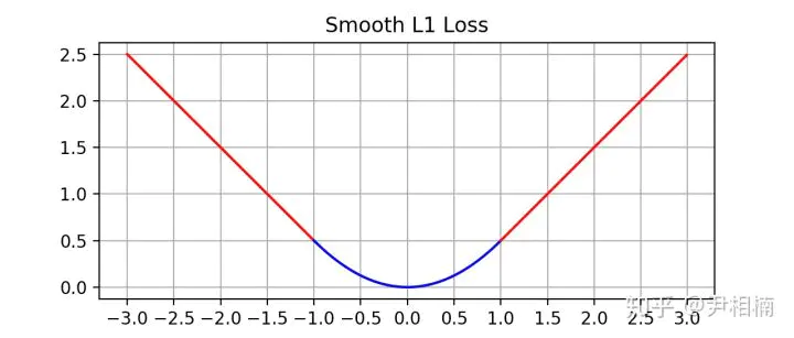
位置回归使用的是smooth L1 loss，通过positive mask实现只取target positive anchor和对应的predicted anchors计算regressive loss

$smooth_{L_1(x)} = \left\{\begin{matrix} 0.5x^2 & if \left | x \right | \lt 1\\ \left | x \right | - 0.5 & otherwise \end{matrix}\right.$

分类损失使用的是binary cross entropy loss,只取positive/negative target loss计算。
$L_i = y_{true}log y_{pred} + (1-y_{true})log(1-y_{pred})$

def losses(self,anchors: List[Boxes],pred_objectness_logits: List[torch.Tensor],gt_labels: List[torch.Tensor],pred_anchor_deltas: List[torch.Tensor],gt_boxes: List[torch.Tensor],
) -> Dict[str, torch.Tensor]:num_images = len(gt_labels)gt_labels = torch.stack(gt_labels)  # (N, sum(Hi*Wi*Ai))# Log the number of positive/negative anchors per-image that's used in trainingpos_mask = gt_labels == 1num_pos_anchors = pos_mask.sum().item()num_neg_anchors = (gt_labels == 0).sum().item()storage = get_event_storage()storage.put_scalar("rpn/num_pos_anchors", num_pos_anchors / num_images)storage.put_scalar("rpn/num_neg_anchors", num_neg_anchors / num_images)localization_loss = _dense_box_regression_loss(anchors,self.box2box_transform,pred_anchor_deltas,gt_boxes,pos_mask,box_reg_loss_type=self.box_reg_loss_type,smooth_l1_beta=self.smooth_l1_beta,)valid_mask = gt_labels >= 0objectness_loss = F.binary_cross_entropy_with_logits(cat(pred_objectness_logits, dim=1)[valid_mask],gt_labels[valid_mask].to(torch.float32),reduction="sum",)normalizer = self.batch_size_per_image * num_imageslosses = {"loss_rpn_cls": objectness_loss / normalizer,# The original Faster R-CNN paper uses a slightly different normalizer# for loc loss. But it doesn't matter in practice"loss_rpn_loc": localization_loss / normalizer,}losses = {k: v * self.loss_weight.get(k, 1.0) for k, v in losses.items()}return losses