建立信用评分模型

读取数据

import numpy as np
import pandas as pd
import matplotlib.pyplot as plt
import seaborn as sns
from sklearn.linear_model import LogisticRegression as LR
from sklearn.ensemble import RandomForestRegressor as rfr
from sklearn.model_selection import train_test_split
from imblearn.over_sampling import SMOTE
%matplotlib inline
data=pd.read_csv('./ch17_cs_training.csv')
data.head()

观察数据

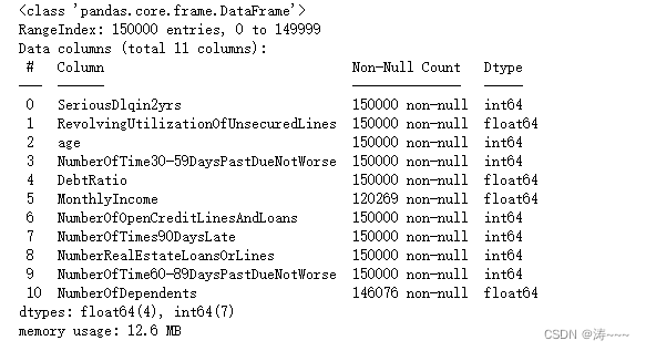
data.info()

在这里插入图片描述

试探性去除重复值，看看数据量是否减少，减少则有重复值，并已去除

data.drop_duplicates(inplace=True) 
data.info()

在这里插入图片描述

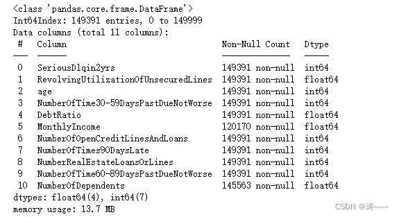
恢复索引，并探索缺失值比例

data.reset_index(inplace=True,drop=True)   
data.isnull().mean()

在这里插入图片描述

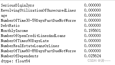
由上可知，家属人数缺失值较少，可直接用均值替换缺失值

data['NumberOfDependents'].fillna(data['NumberOfDependents'].mean(),inplace=True)

由上上可知，月收入缺失值较大，可使用随机森林补充缺失值

def fill_missing_rf(X,y,to_fill):"""使用随机森林填补一个特征的缺失值的函数参数：X：要填补的特征矩阵y：没有缺失值的那部分数据所对应的标签to_fill：要填补的特征"""#构建新特征矩阵和新标签df = X.copy()fill = df.loc[:,to_fill]df = pd.concat([df.loc[:,df.columns != to_fill],pd.DataFrame(y)],axis=1)# 找出我们的训练集和测试集Ytrain = fill[fill.notnull()]Ytest = fill[fill.isnull()]Xtrain = df.iloc[Ytrain.index,:]Xtest = df.iloc[Ytest.index,:]#用随机森林回归来填补缺失值from sklearn.ensemble import RandomForestRegressor as rfrrfr = rfr(n_estimators=100)rfr = rfr.fit(Xtrain, Ytrain)Y_predict = rfr.predict(Xtest)return  Y_predict  X = data.iloc[:,1:] 
y = data.iloc[:,0] 
# 把 X,y 和 含有缺失值的特征 to_fill带入定义好的函数里面
y_pred = fill_missing_rf(X,y,'MonthlyIncome') 
# 将预测的缺失值进行填补
data.loc[data.loc[:,'MonthlyIncome'].isnull(),'MonthlyIncome'] = y_pred

缺失值补充完后，接下来是异常值处理

data.describe([0.01,0.1,0.25,0.5,0.75,0.9,0.99]).T

在这里插入图片描述

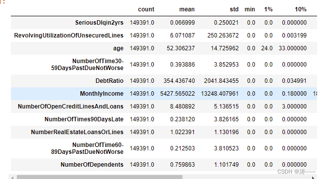
观察到年龄的最小值为0，这不符合银行的业务需求，直接删掉

data = data[data["age"] != 0]

继续观察有三个指标看起来很奇怪：

“NumberOfTime30-59DaysPastDueNotWorse”
“NumberOfTime60-89DaysPastDueNotWorse”
“NumberOfTimes90DaysLate”
这三个指标分别是“过去两年内出现35-59天逾期但是没有发展的更坏的次数”，“过去两年内出现60-89天逾期但是没
有发展的更坏的次数”,“过去两年内出现90天逾期的次数”。这三个指标，在99%的分布的时候依然是2，最大值却是
98,看起来很不正常。

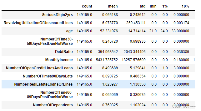
data[data.loc[:,"NumberOfTimes90DaysLate"] > 90].count()

不对劲，接着判断

有225个样本存在这样的情况，并且这些样本，我们观察一下，标签并不都是1，他们并不都是坏客户这显然是不正常的。
因此，我们基本可以判断，这些样本是某种异常，应该把它们删除。

data = data[data.loc[:,'NumberOfTimes90DaysLate']<90]

检测

data.describe([0.01,0.1,0.25,0.5,0.75,0.9,0.99]).T

在这里插入图片描述

恢复索引，并探索标签的分布

data.reset_index(inplace=True,drop=True) 
X = data.iloc[:,1:] 
y = data.iloc[:,0]
# y.value_counts() 
sns.countplot(x="SeriousDlqin2yrs", data=data) 
n_1_sample = y.value_counts()[1]
n_0_sample = y.value_counts()[0] 
print('样本个数：{};1占{:.2%};0占{:.2%}'.format(len(y),n_1_sample/len(y),n_0_sample/len(y)))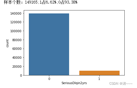

在这里插入图片描述

数据不平衡，让它平衡

#在逻辑回归中，使用最多的是上采样法SMOTE进行 样本均衡import imblearn
#imblearn是专门用来处理不平衡数据集的库，在处理样本不均衡问题中性能高过sklearn很多
#imblearn里面也是一个个的类，也需要进行实例化，fit拟合，和sklearn用法相似
from imblearn.over_sampling import SMOTE
sm = SMOTE(random_state=42) #实例化
X,y = sm.fit_resample(X,y) #返回已经上采样完毕后的特征矩阵和标签
n_sample_ = X.shape[0]
n_1_sample = pd.Series(y).value_counts()[1]
n_0_sample = pd.Series(y).value_counts()[0]
print('样本个数：{}; 1占{:.2%}; 0占{:.2%}'.format(n_sample_,n_1_sample/n_sample_,n_0_sample/n_sample_))

训练数据构建模型

from sklearn.model_selection import train_test_split
X = pd.DataFrame(X)
y = pd.DataFrame(y)X_train, X_vali, Y_train, Y_vali = train_test_split(X,y,test_size=0.3,random_state=420) 
model_data = pd.concat([Y_train, X_train], axis=1)
model_data.reset_index(drop=True,inplace=True)
model_data.columns = data.columns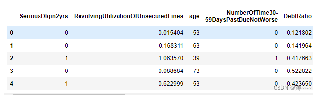

在这里插入图片描述

划分训练集和验证集

vali_data = pd.concat([Y_vali, X_vali], axis=1)
vali_data.reset_index(drop=True,inplace=True) 
vali_data.columns = data.columns
model_data.to_csv(r'.\model_data.csv')
vali_data.to_csv(r'.\vali_data.csv')

分析训练集

import matplotlib.pyplot as plt
from pylab import mpl
mpl.rcParams['font.sans-serif'] = ['SimHei']
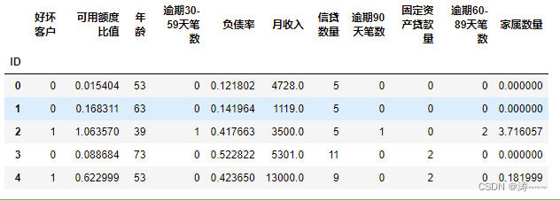
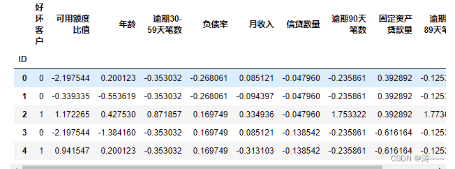
df=pd.read_csv(r'.\model_data.csv', index_col = 0)
df.index.name = 'ID'
states={'SeriousDlqin2yrs':'好坏客户','RevolvingUtilizationOfUnsecuredLines':'可用额度比值','age':'年龄','NumberOfTime30-59DaysPastDueNotWorse':'逾期30-59天笔数','DebtRatio':'负债率','MonthlyIncome':'月收入','NumberOfOpenCreditLinesAndLoans':'信贷数量','NumberOfTimes90DaysLate':'逾期90天笔数','NumberRealEstateLoansOrLines':'固定资产贷款量','NumberOfTime60-89DaysPastDueNotWorse':'逾期60-89天笔数','NumberOfDependents':'家属数量'}
df.rename(columns=states,inplace=True)
df.head()

在这里插入图片描述

单变量分析

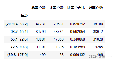
age_cut=pd.cut(df['年龄'],5)
age_cut_group=df['好坏客户'].groupby(age_cut).count()
age_cut_grouped1=df["好坏客户"].groupby(age_cut).sum()
df2=pd.merge(pd.DataFrame(age_cut_group),pd.DataFrame(age_cut_grouped1),left_index=True,right_index=True)
df2.rename(columns={'好坏客户_x':'总客户数','好坏客户_y':'坏客户数'},inplace=True)
df2.insert(2,"好客户数",df2["总客户数"]-df2["坏客户数"])
df2.insert(2,"坏客户占比",df2["坏客户数"]/df2["总客户数"])
df2

在这里插入图片描述

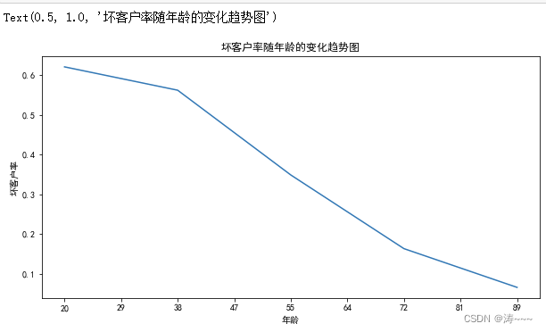
坏客户率随年龄的变化趋势图

ax11=df2["坏客户占比"].plot(figsize=(10,5))
ax11.set_xticklabels([0,20,29,38,47,55,64,72,81,89,98,107])
ax11.set_ylabel("坏客户率")
ax11.set_title("坏客户率随年龄的变化趋势图")

在这里插入图片描述

多变量分析

import seaborn as sns
corr = df.corr()#计算各变量的相关性系数
xticks = list(corr.index)#x轴标签
yticks = list(corr.index)#y轴标签
fig = plt.figure(figsize=(15,10))
ax1 = fig.add_subplot(1, 1, 1)
sns.heatmap(corr, annot=True, cmap="rainbow",ax=ax1,linewidths=.5, annot_kws={'size': 9, 'weight': 'bold', 'color': 'blue'})
ax1.set_xticklabels(xticks, rotation=35, fontsize=15)
ax1.set_yticklabels(yticks, rotation=0, fontsize=15)
plt.show()

在这里插入图片描述

WOE分箱和WOE值计算

cut1=pd.qcut(df["可用额度比值"],4,labels=False)
cut2=pd.qcut(df["年龄"],8,labels=False)
bins3=[-1,0,1,3,5,13]
cut3=pd.cut(df["逾期30-59天笔数"],bins3,labels=False)
cut4=pd.qcut(df["负债率"],3,labels=False)
cut5=pd.qcut(df["月收入"],4,labels=False)
cut6=pd.qcut(df["信贷数量"],4,labels=False)
bins7=[-1, 0, 1, 3,5, 20]
cut7=pd.cut(df["逾期90天笔数"],bins7,labels=False)
bins8=[-1, 0,1,2, 3, 33]
cut8=pd.cut(df["固定资产贷款量"],bins8,labels=False)
bins9=[-1, 0, 1, 3, 12]
cut9=pd.cut(df["逾期60-89天笔数"],bins9,labels=False)
bins10=[-1, 0, 1, 2, 3, 5, 21]
cut10=pd.cut(df["家属数量"],bins10,labels=False)rate=df["好坏客户"].sum()/(df["好坏客户"].count()-df["好坏客户"].sum())
def get_woe_data(cut):grouped=df["好坏客户"].groupby(cut,as_index = True).value_counts()woe=np.log(grouped.unstack().iloc[:,1]/grouped.unstack().iloc[:,0]/rate)return woe
cut1_woe=get_woe_data(cut1)
cut2_woe=get_woe_data(cut2)
cut3_woe=get_woe_data(cut3)
cut4_woe=get_woe_data(cut4)
cut5_woe=get_woe_data(cut5)
cut6_woe=get_woe_data(cut6)
cut7_woe=get_woe_data(cut7)
cut8_woe=get_woe_data(cut8)
cut9_woe=get_woe_data(cut9)
cut10_woe=get_woe_data(cut10)

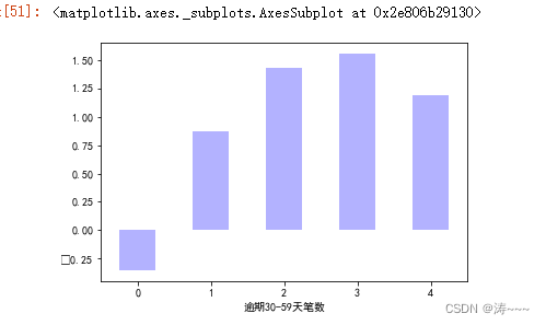
随便挑几个变量看下woe

可更改变量名来查看

# cut1_woe.plot.bar(color='b',alpha=0.3,rot=0)
# cut2_woe.plot.bar(color='b',alpha=0.3,rot=0)
cut3_woe.plot.bar(color='b',alpha=0.3,rot=0)

在这里插入图片描述

IV值计算

def get_IV_data(cut,cut_woe):grouped=df["好坏客户"].groupby(cut,as_index = True).value_counts()cut_IV=((grouped.unstack().iloc[:,1]/df["好坏客户"].sum()-grouped.unstack().iloc[:,0]/(df["好坏客户"].count()-df["好坏客户"].sum()))*cut_woe).sum()    return cut_IV
#计算各分组的IV值
cut1_IV=get_IV_data(cut1,cut1_woe)
cut2_IV=get_IV_data(cut2,cut2_woe)
cut3_IV=get_IV_data(cut3,cut3_woe)
cut4_IV=get_IV_data(cut4,cut4_woe)
cut5_IV=get_IV_data(cut5,cut5_woe)
cut6_IV=get_IV_data(cut6,cut6_woe)
cut7_IV=get_IV_data(cut7,cut7_woe)
cut8_IV=get_IV_data(cut8,cut8_woe)
cut9_IV=get_IV_data(cut9,cut9_woe)
cut10_IV=get_IV_data(cut10,cut10_woe)
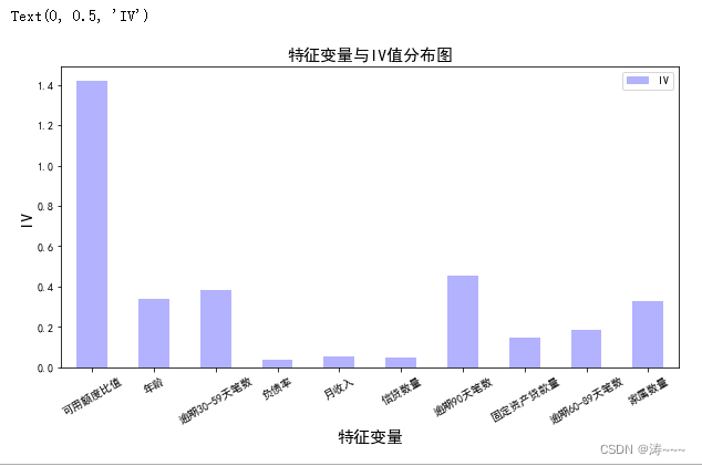
IV=pd.DataFrame([cut1_IV,cut2_IV,cut3_IV,cut4_IV,cut5_IV,cut6_IV,cut7_IV,cut8_IV,cut9_IV,cut10_IV],index=['可用额度比值','年龄','逾期30-59天笔数','负债率','月收入','信贷数量','逾期90天笔数','固定资产贷款量','逾期60-89天笔数','家属数量'],columns=['IV'])
iv=IV.plot.bar(color='b',alpha=0.3,rot=30,figsize=(10,5),fontsize=(10))
iv.set_title('特征变量与IV值分布图',fontsize=(15))
iv.set_xlabel('特征变量',fontsize=(15))
iv.set_ylabel('IV',fontsize=(15))

在这里插入图片描述

WOE值替换

df_new=pd.DataFrame()   #新建df_new存放woe转换后的数据
def replace_data(cut,cut_woe):a=[]for i in cut.unique():a.append(i)a.sort()for m in range(len(a)):cut.replace(a[m],cut_woe.values[m],inplace=True)return cut
df_new["好坏客户"]=df["好坏客户"]
df_new["可用额度比值"]=replace_data(cut1,cut1_woe)
df_new["年龄"]=replace_data(cut2,cut2_woe)
df_new["逾期30-59天笔数"]=replace_data(cut3,cut3_woe)
df_new["负债率"]=replace_data(cut4,cut4_woe)
df_new["月收入"]=replace_data(cut5,cut5_woe)
df_new["信贷数量"]=replace_data(cut6,cut6_woe)
df_new["逾期90天笔数"]=replace_data(cut7,cut7_woe)
df_new["固定资产贷款量"]=replace_data(cut8,cut8_woe)
df_new["逾期60-89天笔数"]=replace_data(cut9,cut9_woe)
df_new["家属数量"]=replace_data(cut10,cut10_woe)
df_new.head()

在这里插入图片描述

训练模型

from sklearn.linear_model import LogisticRegression
from sklearn.model_selection import train_test_split
x=df_new.iloc[:,1:]
y=df_new.iloc[:,:1]
x_train,x_test,y_train,y_test=train_test_split(x,y,test_size=0.6,random_state=0)
model=LogisticRegression()
clf=model.fit(x_train,y_train)
print('测试成绩：{}'.format(clf.score(x_test,y_test)))

测试成绩：0.7791803769069698

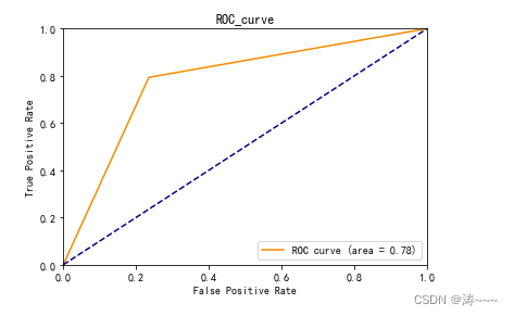
模型评估roc曲线

coe=clf.coef_  
y_pred=clf.predict(x_test)
from sklearn.metrics import roc_curve, auc
fpr, tpr, threshold = roc_curve(y_test, y_pred)
roc_auc = auc(fpr, tpr)
plt.plot(fpr, tpr, color='darkorange',label='ROC curve (area = %0.2f)' % roc_auc)
plt.plot([0, 1], [0, 1], color='navy',  linestyle='--')
plt.xlim([0.0, 1.0])
plt.ylim([0.0, 1.0])
plt.xlabel('False Positive Rate')
plt.ylabel('True Positive Rate')
plt.title('ROC_curve')
plt.legend(loc="lower right")
plt.show()
print(roc_auc)

在这里插入图片描述

绘画KS曲线

fig, ax = plt.subplots()
ax.plot(1 - threshold, tpr, label='tpr') # ks曲线要按照预测概率降序排列，所以需要1-threshold镜像
ax.plot(1 - threshold, fpr, label='fpr')
ax.plot(1 - threshold, tpr-fpr,label='KS')
plt.xlabel('score')
plt.title('KS Curve')
plt.ylim([0.0, 1.0])
plt.figure(figsize=(20,20))
legend = ax.legend(loc='upper left')
plt.show()
print(max(tpr-fpr))

在这里插入图片描述
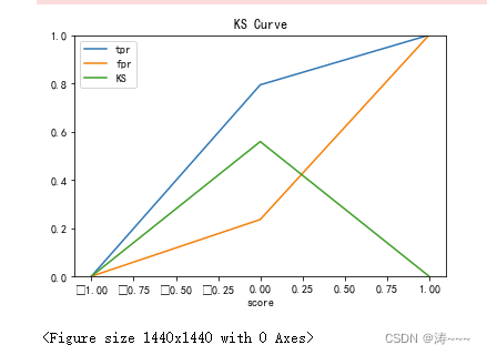
0.5584308938611491

模型结果转评分

factor = 20 / np.log(2)
offset = 600 - 20 * np.log(20) / np.log(2)
def get_score(coe,woe,factor):scores=[]for w in woe:score=round(coe*w*factor,0)scores.append(score)return scores
x1 = get_score(coe[0][0], cut1_woe, factor)
x2 = get_score(coe[0][1], cut2_woe, factor)
x3 = get_score(coe[0][2], cut3_woe, factor)
x4 = get_score(coe[0][3], cut4_woe, factor)
x5 = get_score(coe[0][4], cut5_woe, factor)
x6 = get_score(coe[0][5], cut6_woe, factor)
x7 = get_score(coe[0][6], cut7_woe, factor)
x8 = get_score(coe[0][7], cut8_woe, factor)
x9 = get_score(coe[0][8], cut9_woe, factor)
x10 = get_score(coe[0][9], cut10_woe, factor)
print("可用额度比值对应的分数:{}".format(x1))
print("年龄对应的分数:{}".format(x2))
print("逾期30-59天笔数对应的分数:{}".format(x3))
print("负债率对应的分数:{}".format(x4))
print("月收入对应的分数:{}".format(x5))
print("信贷数量对应的分数:{}".format(x6))
print("逾期90天笔数对应的分数:{}".format(x7))
print("固定资产贷款量对应的分数:{}".format(x8))
print("逾期60-89天笔数对应的分数:{}".format(x9))
print("家属数量对应的分数:{}".format(x10))

计算用户总分

cu1=pd.qcut(df["可用额度比值"],4,labels=False,retbins=True)
bins1=cu1[1]
cu2=pd.qcut(df["年龄"],8,labels=False,retbins=True)
bins2=cu2[1]bins3=[-1,0,1,3,5,13]
cut3=pd.cut(df["逾期30-59天笔数"],bins3,labels=False)
cu4=pd.qcut(df["负债率"],3,labels=False,retbins=True)
bins4=cu4[1]
cu5=pd.qcut(df["月收入"],4,labels=False,retbins=True)
bins5=cu5[1]
cu6=pd.qcut(df["信贷数量"],4,labels=False,retbins=True)
bins6=cu6[1]

对应各评分进行求和

def compute_score(series,bins,score):list = []i = 0while i < len(series):value = series[i]j = len(bins) - 2m = len(bins) - 2while j >= 0:if value >= bins[j]:j = -1else:j -= 1m -= 1list.append(score[m])i += 1return list

代入测试集进行预估

test1 = pd.read_csv(r'.\vali_data.csv')
test1['x1'] = pd.Series(compute_score(test1['RevolvingUtilizationOfUnsecuredLines'], bins1, x1))
test1['x2'] = pd.Series(compute_score(test1['age'], bins2, x2))
test1['x3'] = pd.Series(compute_score(test1['NumberOfTime30-59DaysPastDueNotWorse'], bins3, x3))
test1['x4'] = pd.Series(compute_score(test1['DebtRatio'], bins4, x4))
test1['x5'] = pd.Series(compute_score(test1['MonthlyIncome'], bins5, x5))
test1['x6'] = pd.Series(compute_score(test1['NumberOfOpenCreditLinesAndLoans'], bins6, x6))
test1['x7'] = pd.Series(compute_score(test1['NumberOfTimes90DaysLate'], bins7, x7))
test1['x8'] = pd.Series(compute_score(test1['NumberRealEstateLoansOrLines'], bins8, x8))
test1['x9'] = pd.Series(compute_score(test1['NumberOfTime60-89DaysPastDueNotWorse'], bins9, x9))
test1['x10'] = pd.Series(compute_score(test1['NumberOfDependents'], bins10, x10))
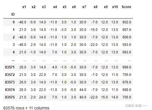
test1['Score'] = test1['x1']+test1['x2']+test1['x3']+test1['x4']+test1['x5']+test1['x6']+test1['x7']+test1['x8']+test1['x9']+test1['x10']+600
test1.to_csv(r'./ScoreData.csv', index=False)

查看测试集结果

Score = pd.read_csv(r'.\ScoreData.csv',index_col=0)
Score.index.name = 'ID'
Score.iloc[:,11:23]

在这里插入图片描述