目标检测的基本概念

报名参加datawhale的目标检测组队学习，虽然做objdec有一段时间了，但是还没有系统的记录过自己的学习历程，就借此机会记录一下自己的感想和经历吧，就当是记笔记了。

理解

目标检测实际上也是一种分类算法，利用对整张图的遍历或者anchor来将带有目标的图像输入网络进行分类，并通过loss不断修正bbox的大小形状，从而达到目标检测的效果

实现

截止到目前我理解的one stage的目标检测方式主要是有SSD和yolo，SSD的滑动窗口相当于把单张图像进行一次遍历，从而达到检测所有目标的结果，而yolo则是利用anchor，首先对训练数据集的ground truth进行kmeans，得到bbox最有可能出现的位置，从而进行anchor的投放，随后利用backbone进行bbox图像的分类，并通过iou进行bbox的调整。

目标框的表达形式

目标框的表达形式主要有以下几种，分别为利用左上角，右下角[x1,y1,x2,y2]，和yolo用的[x,y,w,h]这种格式，而yolo在标签存储过程中，往往将标签的值进行归一化，公式为x = left_x/imgsz, y = top_y/imgsz, w = w/imgsz, h = h/imgsz。

两种格式转换代码

def xy_to_cxcy(xy):"""Convert bounding boxes from boundary coordinates (x_min, y_min, x_max, y_max) to center-size coordinates (c_x, c_y, w, h).:param xy: bounding boxes in boundary coordinates, a tensor of size (n_boxes, 4):return: bounding boxes in center-size coordinates, a tensor of size (n_boxes, 4)"""return torch.cat([(xy[:, 2:] + xy[:, :2]) / 2,  # c_x, c_yxy[:, 2:] - xy[:, :2]], 1)  # w, hdef cxcy_to_xy(cxcy):"""Convert bounding boxes from center-size coordinates (c_x, c_y, w, h) to boundary coordinates (x_min, y_min, x_max, y_max).:param cxcy: bounding boxes in center-size coordinates, a tensor of size (n_boxes, 4):return: bounding boxes in boundary coordinates, a tensor of size (n_boxes, 4)"""return torch.cat([cxcy[:, :2] - (cxcy[:, 2:] / 2),  # x_min, y_mincxcy[:, :2] + (cxcy[:, 2:] / 2)], 1)  # x_max, y_max

交并比（IoU）

IoU的全称是交并比（Intersection over Union），表示两个目标框的交集占其并集的比例，交并比经过发展，分为giou，diou，ciou，近期在ECCV’ 20上的PIoU Loss: Towards Accurate Oriented Object Detection in Complex Environments还提出了piou的概念，由于还没学习piou，这里就不再讲述，将在接下来的每日一网的计划中进行系统学习。
简单来说，iou就是两个bbox的交集与并集的比值，用图片来表示就是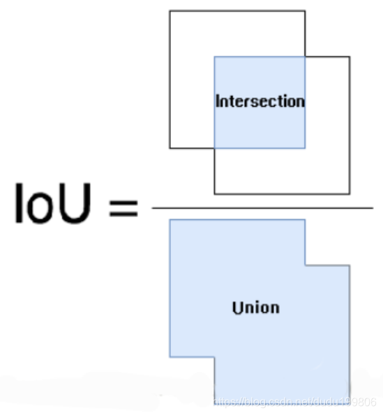
具体的计算流程大概是这样的

1.首先获取两个框的坐标，红框坐标: 左上(red_x1, red_y1), 右下(red_x2, red_y2)，绿框坐标: 左上(green_x1, green_y1)，右下(green_x2, green_y2)
2.计算两个框左上点的坐标最大值:(max(red_x1, green_x1), max(red_y1, green_y1)), 和右下点坐标最小值:(min(red_x2, green_x2), min(red_y2, green_y2))
3.利用2算出的信息计算黄框面积：yellow_area
4.计算红绿框的面积：red_area 和 green_area
5.iou = yellow_area / (red_area + green_area - yellow_area)

代码表示：

def find_intersection(set_1, set_2):""" Find the intersection of every box combination between two sets of boxes that are in boundary coordinates.:param set_1: set 1, a tensor of dimensions (n1, 4)                                                                                                           :param set_2: set 2, a tensor of dimensions (n2, 4):return: intersection of each of the boxes in set 1 with respect to each of the boxes in set 2, a tensor of dimensions (n1, n2)"""# PyTorch auto-broadcasts singleton dimensionslower_bounds = torch.max(set_1[:, :2].unsqueeze(1), set_2[:, :2].unsqueeze(0))  # (n1, n2, 2)upper_bounds = torch.min(set_1[:, 2:].unsqueeze(1), set_2[:, 2:].unsqueeze(0))  # (n1, n2, 2)intersection_dims = torch.clamp(upper_bounds - lower_bounds, min=0)  # (n1, n2, 2)return intersection_dims[:, :, 0] * intersection_dims[:, :, 1]  # (n1, n2)def find_jaccard_overlap(set_1, set_2):""" Find the Jaccard Overlap (IoU) of every box combination between two sets of boxes that are in boundary coordinates.:param set_1: set 1, a tensor of dimensions (n1, 4):param set_2: set 2, a tensor of dimensions (n2, 4):return: Jaccard Overlap of each of the boxes in set 1 with respect to each of the boxes in set 2, a tensor of dimensions (n1, n2)"""# Find intersectionsintersection = find_intersection(set_1, set_2)  # (n1, n2)# Find areas of each box in both setsareas_set_1 = (set_1[:, 2] - set_1[:, 0]) * (set_1[:, 3] - set_1[:, 1])  # (n1)areas_set_2 = (set_2[:, 2] - set_2[:, 0]) * (set_2[:, 3] - set_2[:, 1])  # (n2)# Find the union# PyTorch auto-broadcasts singleton dimensionsunion = areas_set_1.unsqueeze(1) + areas_set_2.unsqueeze(0) - intersection  # (n1, n2)return intersection / union  # (n1, n2)

GIoU 作为 IoU 的升级版，既继承了 IoU 的两个优点，又弥补了 IoU 无法衡量无重叠框之间的距离的缺点。具体计算方式是在 IoU 计算的基础上寻找一个 smallest convex shapes C，具体计算公式是：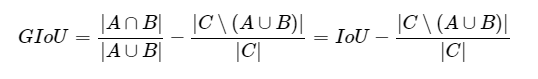
下图中有两个不同的检测结果 bad & better，不难看出距离 gt box 越远 C 越大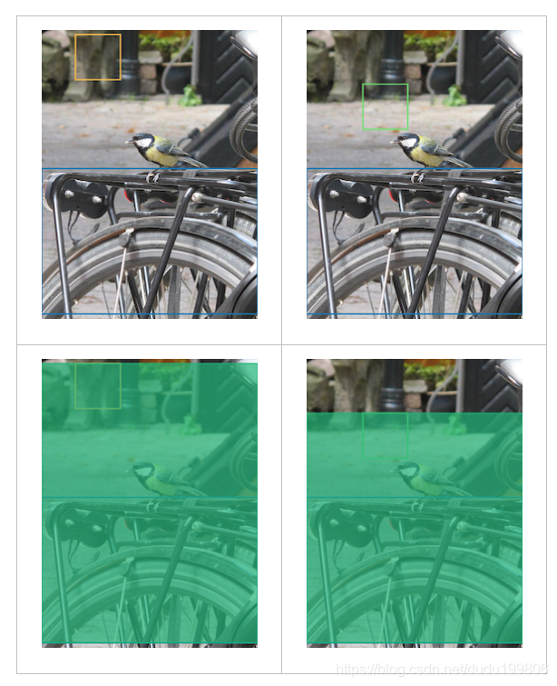
DIoU要比GIou更加符合目标框回归的机制，将目标与anchor之间的距离，重叠率以及尺度都考虑进去，使得目标框回归变得更加稳定，不会像IoU和GIoU一样出现训练过程中发散等问题。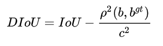
其中， b， bgt 分别代表了预测框和真实框的中心点，且 p代表的是计算两个中心点间的欧式距离。c代表的是能够同时包含预测框和真实框的最小闭包区域的对角线距离。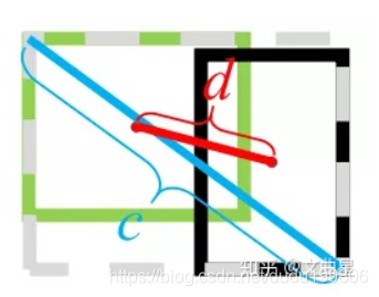
与GIoU loss类似，DIoU loss（ [公式] ）在与目标框不重叠时，仍然可以为边界框提供移动方向。
DIoU loss可以直接最小化两个目标框的距离，因此比GIoU loss收敛快得多。
对于包含两个框在水平方向和垂直方向上这种情况，DIoU损失可以使回归非常快，而GIoU损失几乎退化为IoU损失。
DIoU还可以替换普通的IoU评价策略，应用于NMS中，使得NMS得到的结果更加合理和有效。

ciou
论文考虑到bbox回归三要素中的长宽比还没被考虑到计算中，因此，进一步在DIoU的基础上提出了CIoU。
这里因为不会打公式，引用一下知乎大佬的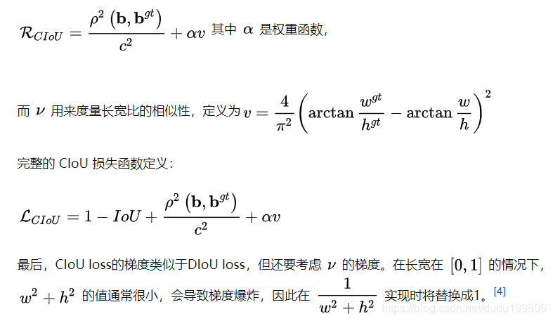

voc数据集

下载

官网下载：http://host.robots.ox.ac.uk/pascal/VOC/
百度网盘：https://pan.baidu.com/s/1SM2M6S366igDriiCWGyhDg
提取码：7aek
下载后放到dataset目录下解压即可

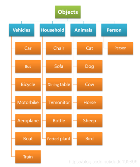
数据集类别

数据集分为4个大类　20个小类

VOC数量集图像和目标数量的基本信息如下图所示:

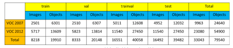
其中，Images表示图片数量，Objects表示目标数量
将下载得到的压缩包解压，可以得到如图3-9所示的一系列文件夹，由于VOC数据集不仅被拿来做目标检测，也可以拿来做分割等任务，因此除了目标检测所需的文件之外，还包含分割任务所需的文件，比如SegmentationClass,SegmentationObject，这里，我们主要对目标检测任务涉及到的文件进行介绍。

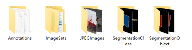
1.JPEGImages

这个文件夹中存放所有的图片，包括训练验证测试用到的所有图片。

2.ImageSets

这个文件夹中包含三个子文件夹，Layout、Main、Segmentation

Layout文件夹中存放的是train，valid，test和train+valid数据集的文件名

Segmentation文件夹中存放的是分割所用train，valid，test和train+valid数据集的文件名

Main文件夹中存放的是各个类别所在图片的文件名，比如cow_val，表示valid数据集中，包含有cow类别目标的图片名称。

3.Annotations

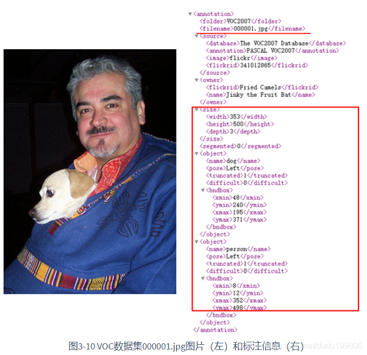
Annotation文件夹中存放着每张图片相关的标注信息，以xml格式的文件存储，可以通过记事本或者浏览器打开，我们以000001.jpg这张图片为例说明标注文件中各个属性的含义，见图3-10。

。

1.filename：图片名称

2.size：图片宽高，

3.depth表示图片通道数

4.object：表示目标，包含下面两部分内容。

首先是目标类别name为dog。pose表示目标姿势为left，truncated表示是否是一个被截断的目标，1表示是，0表示不是，在这个例子中，只露出狗头部分，所以truncated为1。difficult为0表示此目标不是一个难以识别的目标。

然后就是目标的bbox信息，可以看到，这里是以[xmin,ymin,xmax,ymax]格式进行标注的，分别表示dog目标的左上角和右下角坐标。

5.一张图片中有多少需要识别的目标，其xml文件中就有多少个object。上面的例子中有两个object，分别对应人和狗。

voc数据集dataloader的构建

1.数据集的准备

根据上面的介绍可以看出，VOC数据集的存储格式还是比较复杂的，为了后面训练中的读取代码更加简洁，这里我们准备了一个预处理脚本create_data_lists.py。

该脚本的作用是进行一系列的数据准备工作，主要是提前将记录标注信息的xml文件(Annotations)进行解析，并将信息整理到json文件之中，这样在运行训练脚本时，只需简单的从json文件中读取已经按想要的格式存储好的标签信息即可。

注: 这样的预处理并不是必须的，和算法或数据集本身均无关系，只是取决于开发者的代码习惯，不同检测框架的处理方法也是不一致的。

可以看到，create_data_lists.py脚本仅有几行代码，其内部调用了utils.py中的create_data_lists方法：

"""pythoncreate_data_lists
"""
from utils import create_data_listsif __name__ == '__main__':# voc07_path，voc12_path为我们训练测试所需要用到的数据集，output_folder为我们生成构建dataloader所需文件的路径# 参数中涉及的路径以个人实际路径为准，建议将数据集放到dataset目录下，和教程保持一致create_data_lists(voc07_path='../../../dataset/VOCdevkit/VOC2007',voc12_path='../../../dataset/VOCdevkit/VOC2012',output_folder='../../../dataset/VOCdevkit')

设置好对应路径后，我们运行数据集准备脚本:

tiny_detector_demo$ python create_data_lists.py

很快啊！dataset/VOCdevkit目录下就生成了若干json文件，这些文件会在后面训练中真正被用到。

不妨手动打开这些json文件，看下都记录了哪些信息。

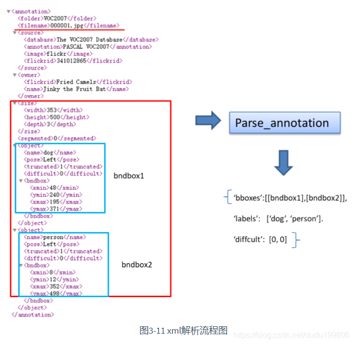
下面来介绍一下parse_annotation函数内部都做了什么，json中又记录了哪些信息。这部分作为选学，不感兴趣可以跳过，只要你已经明确了json中记录的信息的含义。

代码阅读可以参照注释，建议配图3-11一起食用：

"""pythonxml文件解析
"""import json
import os
import torch
import random
import xml.etree.ElementTree as ET    #解析xml文件所用工具
import torchvision.transforms.functional as FT#GPU设置
device = torch.device("cuda" if torch.cuda.is_available() else "cpu")# Label map
#voc_labels为VOC数据集中20类目标的类别名称
voc_labels = ('aeroplane', 'bicycle', 'bird', 'boat', 'bottle', 'bus', 'car', 'cat', 'chair', 'cow', 'diningtable','dog', 'horse', 'motorbike', 'person', 'pottedplant', 'sheep', 'sofa', 'train', 'tvmonitor')#创建label_map字典，用于存储类别和类别索引之间的映射关系。比如：{1：'aeroplane'， 2：'bicycle'，......}
label_map = {k: v + 1 for v, k in enumerate(voc_labels)}
#VOC数据集默认不含有20类目标中的其中一类的图片的类别为background，类别索引设置为0
label_map['background'] = 0#将映射关系倒过来，{类别名称：类别索引}
rev_label_map = {v: k for k, v in label_map.items()}  # Inverse mapping#解析xml文件，最终返回这张图片中所有目标的标注框及其类别信息，以及这个目标是否是一个difficult目标
def parse_annotation(annotation_path):#解析xmltree = ET.parse(annotation_path)root = tree.getroot()boxes = list()    #存储bboxlabels = list()    #存储bbox对应的labeldifficulties = list()    #存储bbox对应的difficult信息#遍历xml文件中所有的object，前面说了，有多少个object就有多少个目标for object in root.iter('object'):#提取每个object的difficult、label、bbox信息difficult = int(object.find('difficult').text == '1')label = object.find('name').text.lower().strip()if label not in label_map:continuebbox = object.find('bndbox')xmin = int(bbox.find('xmin').text) - 1ymin = int(bbox.find('ymin').text) - 1xmax = int(bbox.find('xmax').text) - 1ymax = int(bbox.find('ymax').text) - 1#存储boxes.append([xmin, ymin, xmax, ymax])labels.append(label_map[label])difficulties.append(difficult)#返回包含图片标注信息的字典return {'boxes': boxes, 'labels': labels, 'difficulties': difficulties}

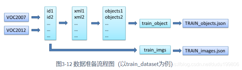
接下来看一下create_data_lists函数在做什么，建议配图3-12一起食用：

"""python分别读取train和valid的图片和xml信息，创建用于训练和测试的json文件
"""
def create_data_lists(voc07_path, voc12_path, output_folder):"""Create lists of images, the bounding boxes and labels of the objects in these images, and save these to file.:param voc07_path: path to the 'VOC2007' folder:param voc12_path: path to the 'VOC2012' folder:param output_folder: folder where the JSONs must be saved"""#获取voc2007和voc2012数据集的绝对路径voc07_path = os.path.abspath(voc07_path)voc12_path = os.path.abspath(voc12_path)train_images = list()train_objects = list()n_objects = 0# Training datafor path in [voc07_path, voc12_path]:# Find IDs of images in training data#获取训练所用的train和val数据的图片idwith open(os.path.join(path, 'ImageSets/Main/trainval.txt')) as f:ids = f.read().splitlines()#根据图片id，解析图片的xml文件，获取标注信息for id in ids:# Parse annotation's XML fileobjects = parse_annotation(os.path.join(path, 'Annotations', id + '.xml'))if len(objects['boxes']) == 0:    #如果没有目标则跳过continuen_objects += len(objects)        #统计目标总数train_objects.append(objects)    #存储每张图片的标注信息到列表train_objectstrain_images.append(os.path.join(path, 'JPEGImages', id + '.jpg'))    #存储每张图片的路径到列表train_images，用于读取图片assert len(train_objects) == len(train_images)        #检查图片数量和标注信息量是否相等，相等才继续执行程序# Save to file#将训练数据的图片路径，标注信息，类别映射信息，分别保存为json文件with open(os.path.join(output_folder, 'TRAIN_images.json'), 'w') as j:json.dump(train_images, j)with open(os.path.join(output_folder, 'TRAIN_objects.json'), 'w') as j:json.dump(train_objects, j)with open(os.path.join(output_folder, 'label_map.json'), 'w') as j:json.dump(label_map, j)  # save label map tooprint('\nThere are %d training images containing a total of %d objects. Files have been saved to %s.' % (len(train_images), n_objects, os.path.abspath(output_folder)))#与Train data一样，目的是将测试数据的图片路径，标注信息，类别映射信息，分别保存为json文件，参考上面的注释理解# Test datatest_images = list()test_objects = list()n_objects = 0# Find IDs of images in the test datawith open(os.path.join(voc07_path, 'ImageSets/Main/test.txt')) as f:ids = f.read().splitlines()for id in ids:# Parse annotation's XML fileobjects = parse_annotation(os.path.join(voc07_path, 'Annotations', id + '.xml'))if len(objects) == 0:continuetest_objects.append(objects)n_objects += len(objects)test_images.append(os.path.join(voc07_path, 'JPEGImages', id + '.jpg'))assert len(test_objects) == len(test_images)# Save to filewith open(os.path.join(output_folder, 'TEST_images.json'), 'w') as j:json.dump(test_images, j)with open(os.path.join(output_folder, 'TEST_objects.json'), 'w') as j:json.dump(test_objects, j)print('\nThere are %d test images containing a total of %d objects. Files have been saved to %s.' % (len(test_images), n_objects, os.path.abspath(output_folder)))

到这里，我们的训练数据就准备好了，接下来开始一步步构建训练所需的dataloader

构建dataloader

下面开始介绍构建dataloader的相关代码:

1.首先了解一下训练的时候在哪里定义了dataloader以及是如何定义的。
以下是train.py中的部分代码段：

    #train_dataset和train_loader的实例化train_dataset = PascalVOCDataset(data_folder,split='train',keep_difficult=keep_difficult)train_loader = torch.utils.data.DataLoader(train_dataset, batch_size=batch_size, shuffle=True,collate_fn=train_dataset.collate_fn, num_workers=workers,pin_memory=True)  # note that we're passing the collate function here

可以看到，首先需要实例化PascalVOCDataset类得到train_dataset，然后将train_dataset传入torch.utils.data.DataLoader，进而得到train_loader。

2.接下来看一下PascalVOCDataset是如何定义的。
代码位于 datasets.py 脚本中，可以看到，PascalVOCDataset继承了torch.utils.data.Dataset，然后重写了__init__ , getitem, len 和 collate_fn 四个方法，这也是我们在构建自己的dataset的时候需要经常做的工作，配合下面注释理解代码：

"""pythonPascalVOCDataset具体实现过程
"""
import torch
from torch.utils.data import Dataset
import json
import os
from PIL import Image
from utils import transformclass PascalVOCDataset(Dataset):"""A PyTorch Dataset class to be used in a PyTorch DataLoader to create batches."""#初始化相关变量#读取images和objects标注信息def __init__(self, data_folder, split, keep_difficult=False):""":param data_folder: folder where data files are stored:param split: split, one of 'TRAIN' or 'TEST':param keep_difficult: keep or discard objects that are considered difficult to detect?"""self.split = split.upper()    #保证输入为纯大写字母，便于匹配{'TRAIN', 'TEST'}assert self.split in {'TRAIN', 'TEST'}self.data_folder = data_folderself.keep_difficult = keep_difficult# Read data fileswith open(os.path.join(data_folder, self.split + '_images.json'), 'r') as j:self.images = json.load(j)with open(os.path.join(data_folder, self.split + '_objects.json'), 'r') as j:self.objects = json.load(j)assert len(self.images) == len(self.objects)#循环读取image及对应objects#对读取的image及objects进行tranform操作（数据增广）#返回PIL格式图像，标注框，标注框对应的类别索引，对应的difficult标志(True or False)def __getitem__(self, i):# Read image#*需要注意，在pytorch中，图像的读取要使用Image.open()读取成PIL格式，不能使用opencv#*由于Image.open()读取的图片是四通道的(RGBA)，因此需要.convert('RGB')转换为RGB通道image = Image.open(self.images[i], mode='r')image = image.convert('RGB')# Read objects in this image (bounding boxes, labels, difficulties)objects = self.objects[i]boxes = torch.FloatTensor(objects['boxes'])  # (n_objects, 4)labels = torch.LongTensor(objects['labels'])  # (n_objects)difficulties = torch.ByteTensor(objects['difficulties'])  # (n_objects)# Discard difficult objects, if desired#如果self.keep_difficult为False,即不保留difficult标志为True的目标#那么这里将对应的目标删去if not self.keep_difficult:boxes = boxes[1 - difficulties]labels = labels[1 - difficulties]difficulties = difficulties[1 - difficulties]# Apply transformations#对读取的图片应用transformimage, boxes, labels, difficulties = transform(image, boxes, labels, difficulties, split=self.split)return image, boxes, labels, difficulties#获取图片的总数，用于计算batch数def __len__(self):return len(self.images)#我们知道，我们输入到网络中训练的数据通常是一个batch一起输入，而通过__getitem__我们只读取了一张图片及其objects信息#如何将读取的一张张图片及其object信息整合成batch的形式呢？#collate_fn就是做这个事情，#对于一个batch的images，collate_fn通过torch.stack()将其整合成4维tensor，对应的objects信息分别用一个list存储def collate_fn(self, batch):"""Since each image may have a different number of objects, we need a collate function (to be passed to the DataLoader).This describes how to combine these tensors of different sizes. We use lists.Note: this need not be defined in this Class, can be standalone.:param batch: an iterable of N sets from __getitem__():return: a tensor of images, lists of varying-size tensors of bounding boxes, labels, and difficulties"""images = list()boxes = list()labels = list()difficulties = list()for b in batch:images.append(b[0])boxes.append(b[1])labels.append(b[2])difficulties.append(b[3])#(3,224,224) -> (N,3,224,224)images = torch.stack(images, dim=0)return images, boxes, labels, difficulties  # tensor (N, 3, 224, 224), 3 lists of N tensors each

3.关于数据增强
到这里为止，我们的dataset就算是构建好了，已经可以传给torch.utils.data.DataLoader来获得用于输入网络训练的数据了。

但是不急，构建dataset中有个很重要的一步我们上面只是提及了一下，那就是transform操作(数据增强)。

也就是这一行代码

image, boxes, labels, difficulties = transform(image, boxes, labels, difficulties, split=self.split)

需要注意的是，涉及位置变化的数据增强方法，同样需要对目标框进行一致的处理，因此目标检测框架的数据处理这部分的代码量通常都不小，且比较容易出bug。这里为了降低代码的难度，我们只是使用了几种比较简单的数据增强。

transform 函数的具体代码实现位于 utils.py 中，下面简单进行讲解：

"""pythontransform操作是训练模型中一项非常重要的工作，其中不仅包含数据增强以提升模型性能的相关操作，也包含如数据类型转换(PIL to Tensor)、归一化(Normalize)这些必要操作。
"""
import json
import os
import torch
import random
import xml.etree.ElementTree as ET
import torchvision.transforms.functional as FT"""
可以看到，transform分为TRAIN和TEST两种模式，以本实验为例：在TRAIN时进行的transform有：
1.以随机顺序改变图片亮度，对比度，饱和度和色相，每种都有50％的概率被执行。photometric_distort
2.扩大目标，expand
3.随机裁剪图片，random_crop
4.0.5的概率进行图片翻转，flip
*注意：a. 第一种transform属于像素级别的图像增强，目标相对于图片的位置没有改变，因此bbox坐标不需要变化。但是2，3，4，5都属于图片的几何变化，目标相对于图片的位置被改变，因此bbox坐标要进行相应变化。在TRAIN和TEST时都要进行的transform有：
1.统一图像大小到(224,224)，resize
2.PIL to Tensor
3.归一化，FT.normalize()注1: resize也是一种几何变化，要知道应用数据增强策略时，哪些属于几何变化，哪些属于像素变化
注2: PIL to Tensor操作，normalize操作必须执行
"""def transform(image, boxes, labels, difficulties, split):"""Apply the transformations above.:param image: image, a PIL Image:param boxes: bounding boxes in boundary coordinates, a tensor of dimensions (n_objects, 4):param labels: labels of objects, a tensor of dimensions (n_objects):param difficulties: difficulties of detection of these objects, a tensor of dimensions (n_objects):param split: one of 'TRAIN' or 'TEST', since different sets of transformations are applied:return: transformed image, transformed bounding box coordinates, transformed labels, transformed difficulties"""#在训练和测试时使用的transform策略往往不完全相同，所以需要split变量指明是TRAIN还是TEST时的transform方法assert split in {'TRAIN', 'TEST'}# Mean and standard deviation of ImageNet data that our base VGG from torchvision was trained on# see: https://pytorch.org/docs/stable/torchvision/models.html#为了防止由于图片之间像素差异过大而导致的训练不稳定问题，图片在送入网络训练之间需要进行归一化#对所有图片各通道求mean和std来获得mean = [0.485, 0.456, 0.406]std = [0.229, 0.224, 0.225]new_image = imagenew_boxes = boxesnew_labels = labelsnew_difficulties = difficulties# Skip the following operations for evaluation/testingif split == 'TRAIN':# A series of photometric distortions in random order, each with 50% chance of occurrence, as in Caffe reponew_image = photometric_distort(new_image)# Convert PIL image to Torch tensornew_image = FT.to_tensor(new_image)# Expand image (zoom out) with a 50% chance - helpful for training detection of small objects# Fill surrounding space with the mean of ImageNet data that our base VGG was trained onif random.random() < 0.5:new_image, new_boxes = expand(new_image, boxes, filler=mean)# Randomly crop image (zoom in)new_image, new_boxes, new_labels, new_difficulties = random_crop(new_image, new_boxes, new_labels,new_difficulties)# Convert Torch tensor to PIL imagenew_image = FT.to_pil_image(new_image)# Flip image with a 50% chanceif random.random() < 0.5:new_image, new_boxes = flip(new_image, new_boxes)# Resize image to (224, 224) - this also converts absolute boundary coordinates to their fractional formnew_image, new_boxes = resize(new_image, new_boxes, dims=(224, 224))# Convert PIL image to Torch tensornew_image = FT.to_tensor(new_image)# Normalize by mean and standard deviation of ImageNet data that our base VGG was trained onnew_image = FT.normalize(new_image, mean=mean, std=std)return new_image, new_boxes, new_labels, new_difficulties

4.最后，构建DataLoader
至此，我们已经将VOC数据转换成了dataset，接下来可以用来创建dataloader，这部分pytorch已经帮我们实现好了，我们只需将创建好的dataset送入即可，注意理解相关参数。

"""pythonDataLoader
"""
#参数说明：
#在train时一般设置shufle=True打乱数据顺序，增强模型的鲁棒性
#num_worker表示读取数据时的线程数，一般根据自己设备配置确定（如果是windows系统，建议设默认值0，防止出错）
#pin_memory，在计算机内存充足的时候设置为True可以加快内存中的tensor转换到GPU的速度，具体原因可以百度哈~
train_loader = torch.utils.data.DataLoader(train_dataset, batch_size=batch_size, shuffle=True,collate_fn=train_dataset.collate_fn, num_workers=workers,pin_memory=True)  # note that we're passing the collate function here

小结

到这里，今天的打卡任务就结束了，前半部分是表达了一下想法，后半部分就基本照抄datawhale的代码了，还是需要认真读一下的。明天加油。