keras入门教程

线性回归
非线性模型
MNIST手写数字识别
- 改进
欠拟合，过拟合
- early stop
- Dropout
- 正则化
梯度下降
- 批量梯度下降
- 随机梯度下降
- 小批量梯度下降
- 其他找寻最低点的方法
卷积神经网络
RNN
模型的保存和载入
- 保存模型
- 载入模型
绘制神经网络的结构

几个keras学习的网址：

1.kears官网

2.kears入门指南

我看的是AI MOOC的视频来学习kears框架。

3.keras入门视频链接

入门版视频代码链接

直接看代码是最快的入门方式，这个操作和sklearn机器学习算法基本思想还是一样的。我觉得keras最大的优势在于Sequential,他的层可以一层一层搭建。非常形象。

线性回归

import numpy as np
np.random.seed(1337)   #设置随机数种子
from keras.models import Sequential #Sequential 搭建层的函数
from keras.layers import Dense
import matplotlib.pyplot as plt

# 创建数据集
X = np.linspace(-1, 1, 200)
np.random.shuffle(X)    # 将数据集随机化
Y = 0.5 * X + 2 + np.random.normal(0, 0.05, X.shape) # 假设我们真实模型为：Y=0.5X+2
# 绘制数据集plt.scatter(X, Y) #生成X,Y的散点图
plt.show()

X_train, Y_train = X[:160], Y[:160]     # 把前160个数据放到训练集
X_test, Y_test = X[160:], Y[160:]       # 把后40个点放到测试集

# 定义一个model，
model = Sequential () # Keras有两种类型的模型，序贯模型（Sequential）和函数式模型
                      # 比较常用的是Sequential，它是单输入单输出的
model.add(Dense(1, input_dim=1)) # 通过add()方法一层层添加模型
                                            # Dense是全连接层，第一层需要定义输入，
                                            # 第二层无需指定输入，一般第二层把第一层的输出作为输入

# 定义完模型就需要训练了，不过训练之前我们需要指定一些训练参数
# 通过compile()方法选择损失函数和优化器
# 这里我们用均方误差作为损失函数，随机梯度下降作为优化方法
model.compile(loss='mse', optimizer='sgd')

# 开始训练
print('Training -----------')
for step in range(301):
    cost = model.train_on_batch(X_train, Y_train) # Keras有很多开始训练的函数，这里用train_on_batch（）
    if step % 100 == 0:
        print('train cost: ', cost)

# 测试训练好的模型
print('\nTesting ------------')
cost = model.evaluate(X_test, Y_test, batch_size=40)
print('test cost:', cost)
W, b = model.layers[0].get_weights()    # 查看训练出的网络参数
                                        # 由于我们网络只有一层，且每次训练的输入只有一个，输出只有一个
                                        # 因此第一层训练出Y=WX+B这个模型，其中W,b为训练出的参数
print('Weights=', W, '\nbiases=', b)

# plotting the prediction
Y_pred = model.predict(X_test)
plt.scatter(X_test, Y_test)
plt.plot(X_test, Y_pred)
plt.show()

得到的输出

test cost: 0.0038014401216059923
Weights= [[0.43543226]] 
biases= [1.9983047]

我们实际的曲线为 Y = 0.5 * X + 2 我们预测出来的w=0.435，b=1.99， w相差比较大。所以这个模型并不是很好。可以调整循环次数来提高正确率。

非线性模型

import keras
import numpy as np
import matplotlib.pyplot as plt
# Sequential按顺序构成的模型
from keras.models import Sequential
# Dense全连接层
from keras.layers import Dense,Activation
from keras.optimizers import SGD

# 使用numpy生成200个随机点 
x_data = np.linspace(-0.5,0.5,200)
noise = np.random.normal(0,0.02,x_data.shape)
y_data = np.square(x_data) + noise

# 显示随机点
plt.scatter(x_data,y_data)
plt.show()
# 构建一个顺序模型
model = Sequential()
# 在模型中添加一个全连接层
# 1-10-1
model.add(Dense(units=10,input_dim=1,activation='tanh'))  #如果没有激活函数的话，不能实现非线性。
# model.add(Activation('tanh')) #另一种添加激活函数层的方法
model.add(Dense(units=1,activation='tanh'))
# model.add(Activation('tanh'))
# 定义优化算法
sgd = SGD(lr=0.2) #更改SGD的步长
# sgd:Stochastic gradient descent，随机梯度下降法
# mse:Mean Squared Error，均方误差
model.compile(optimizer=sgd,loss='mse')

# 训练3001个批次
for step in range(6001):
    # 每次训练一个批次
    cost = model.train_on_batch(x_data,y_data)
    # 每500个batch打印一次cost值
    if step % 500 == 0:
        print('cost:',cost)

# x_data输入网络中，得到预测值y_pred
y_pred = model.predict(x_data)

# 显示随机点
plt.scatter(x_data,y_data)
# 显示预测结果
plt.plot(x_data,y_pred,'r-',lw=3)
plt.show()

MNIST手写数字识别


# _*_ coding: utf-8 _*_
# Classifier mnist

import numpy as np

np.random.seed(1337)
from keras.datasets import mnist
from keras.utils import np_utils
from keras.models import Sequential
from keras.layers import Dense, Activation
from keras.optimizers import RMSprop

# 下载数据集
(X_train, y_train), (X_test, y_test) = mnist.load_data()

# 数据预处处理,训练集归一化， 测试集转换成one-hot形式。
#原本shape是[60000,28,28],现在要转成[60000,784], X_train.shape[0]=60000, 后面的参数=-1的话，则就是把后面的两个参数大小相乘。
X_train = X_train.reshape(X_train.shape[0], -1) / 255. #
X_test = X_test.reshape(X_test.shape[0], -1) / 255.
y_train = np_utils.to_categorical(y_train, num_classes=10)
y_test = np_utils.to_categorical(y_test, num_classes=10)

# 不使用model.add()，用以下方式也可以构建网络
# 一定到位，不用一行一行的添加
model = Sequential([
    Dense(400, input_dim=784),#输入维度784, 输出维度400
    Activation('relu'),
    Dense(10), #只有第一层需要填写上输入的维度，后面只需要填写上输出的维度。
    Activation('softmax'),
])

# 定义优化器
# 定义优化器
sgd = SGD(lr=0.2)
model.compile(optimizer=sgd,
              loss='mse',
              metrics=['accuracy'])  # metrics赋值为'accuracy'，会在训练过程中输出正确率

# 这次我们用fit()来训练网路
print('Training ------------')
model.fit(X_train, y_train, epochs=4, batch_size=32)

print('\nTesting ------------')
# 评价训练出的网络
loss, accuracy = model.evaluate(X_test, y_test)

print('test loss: ', loss)
print('test accuracy: ', accuracy)

最后的准确度：

test loss 0.01301875151693821
accuracy 0.917900025844574

准确度只有0.917，精度不是很高。

改进

1.改变损失函数损失函数的选择：如果输出是线性回归模型，损失函数使用二次代价函数；
2.如果输出是S型函数，那么比较适合使用交叉熵代价函数；（交叉熵损失函数经常用于分类问题中，特别是在神经网络做分类问题时，也经常使用交叉熵作为损失函数，此外，由于交叉熵涉及到计算每个类别的概率，所以交叉熵几乎每次都和sigmoid(或softmax)函数一起出现。）
3.如果输出是softmax函数，使用对数代价函数。

因为这个是分类问题，所以可以试试使用交叉熵作为损失函数。改一下优化器的损失函数即可。

# 定义优化器，loss function，训练过程中计算准确率
model.compile(
    optimizer = sgd,
    loss = 'categorical_crossentropy',
    metrics=['accuracy'],
)

最后的准确度：

test loss 0.2678716778755188
accuracy 0.9243999719619751

相比于之前的mse均方误差准确度有所提升。

欠拟合，过拟合

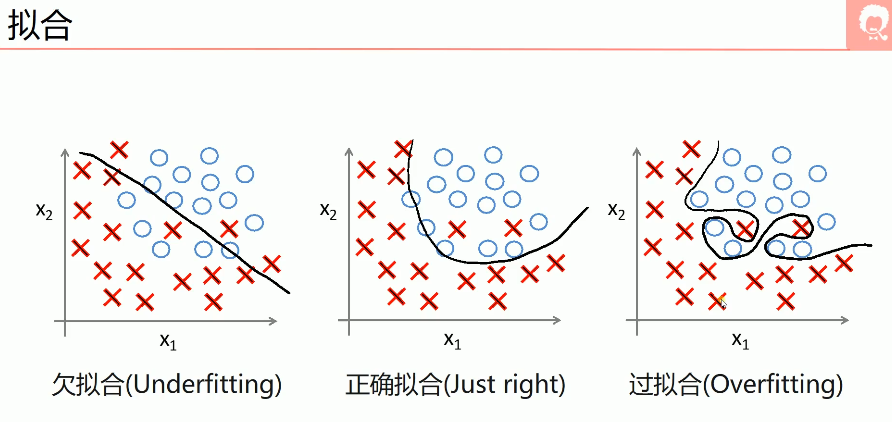
这里就不在赘述这部分内容了。

过拟合的解决方法： 1.dropout

2.增加数据集

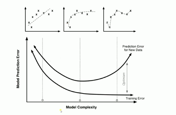
3.early stopping(看上面第二幅图，我们训练到中间那里的时候，就是最好的状态，再训练下去模型越来越差)

4.正则化

early stop

在训练模型的时候，我们往往会设置一个比较大的迭代次数。Early stopping便是一种提前结束训练的策略用来防止过拟合。
一般的做法是记录到目前为止最好的 validation accuracy，当连续10个Epoch没有达到最佳 accuracy时，则可以认为 accuracy不再提高了。此时便可以停止迭代了（Early Stopping）。

体验神经网络训练，可以参考：可以明白各个参数的含义。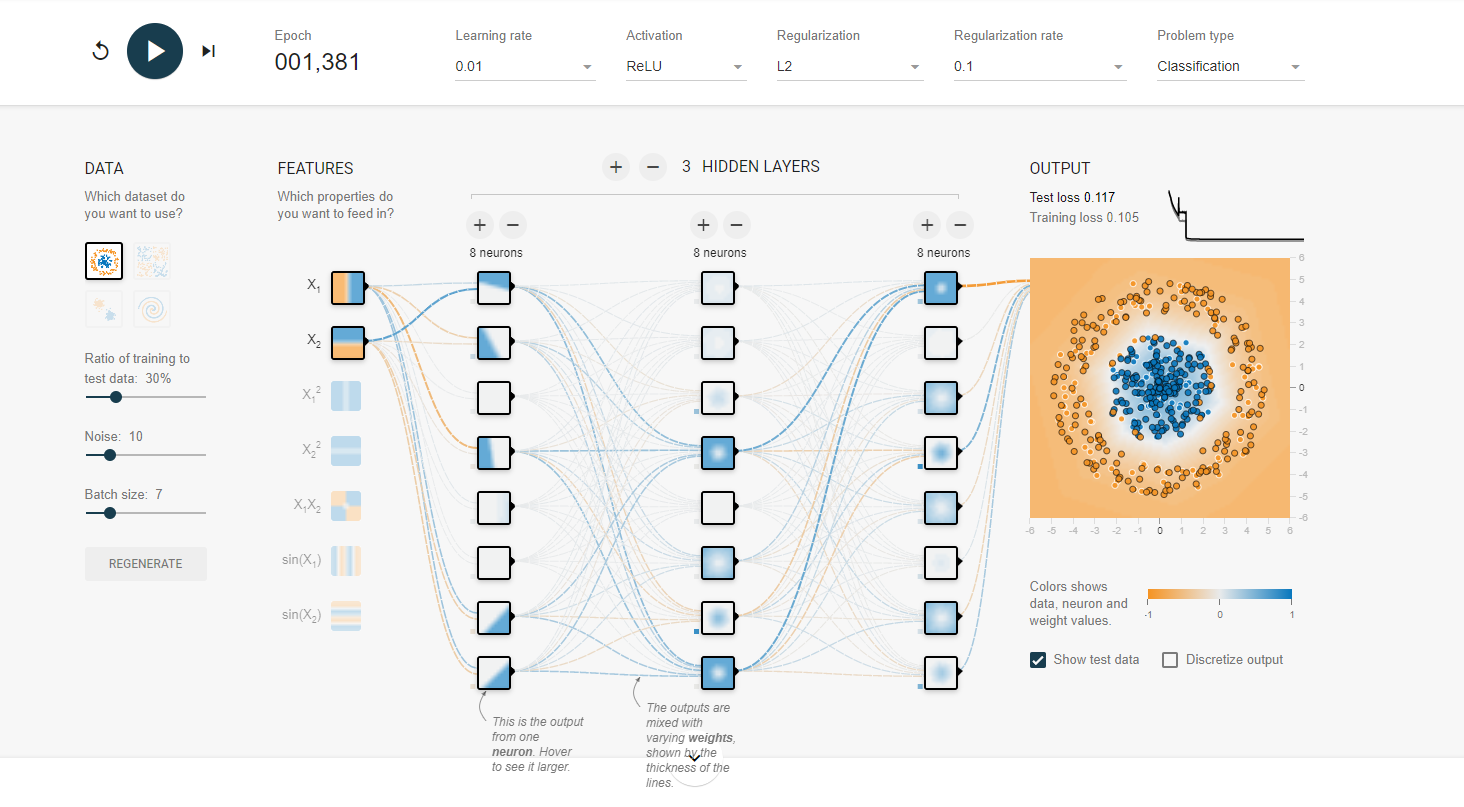

1.A neural network playground

2.回形针paperclip视频

Dropout

1.没有加Dropout

import numpy as np
from keras.datasets import mnist
from keras.utils import np_utils
from keras.models import Sequential
from keras.layers import Dense,Dropout
from keras.optimizers import SGD

# 载入数据
(x_train,y_train),(x_test,y_test) = mnist.load_data()
# (60000,28,28)
print('x_shape:',x_train.shape)
# (60000)
print('y_shape:',y_train.shape)
# (60000,28,28)->(60000,784)
x_train = x_train.reshape(x_train.shape[0],-1)/255.0
x_test = x_test.reshape(x_test.shape[0],-1)/255.0
# 换one hot格式
y_train = np_utils.to_categorical(y_train,num_classes=10)
y_test = np_utils.to_categorical(y_test,num_classes=10)

# 创建模型
model = Sequential([
        Dense(units=200,input_dim=784,bias_initializer='one',activation='tanh'),
     
        Dense(units=100,bias_initializer='one',activation='tanh'),
      
        Dense(units=10,bias_initializer='one',activation='softmax')
    ])

# 定义优化器
sgd = SGD(lr=0.2)

# 定义优化器，loss function，训练过程中计算准确率
model.compile(
    optimizer = sgd,
    loss = 'categorical_crossentropy',
    metrics=['accuracy'],
)

# 训练模型
model.fit(x_train,y_train,batch_size=32,epochs=10)

# 评估模型
loss,accuracy = model.evaluate(x_test,y_test)
print('\ntest loss',loss)
print('test accuracy',accuracy)

loss,accuracy = model.evaluate(x_train,y_train)
print('train loss',loss)
print('train accuracy',accuracy)

输出的准确度：

test loss 0.07081281393766403
test accuracy 0.9785000085830688
1875/1875 [==============================] - 3s 2ms/step - loss: 0.0076 - accuracy: 0.9987
train loss 0.007551191840320826
train accuracy 0.9987166523933411

面对复杂的模型，train accuracy 和 test accuracy相差很大。过拟合现象严重，所以需要加入Dropout层降低过拟合现象。

只需要在层结构中，加入Dropout层即可。

model = Sequential([
        Dense(units=200,input_dim=784,bias_initializer='one',activation='tanh'),
        Dropout(0.4), #每一次让40%的神经元正常工作
        Dense(units=100,bias_initializer='one',activation='tanh'),
        Dropout(0.4),
        Dense(units=10,bias_initializer='one',activation='softmax')
    ])

输出的准确率：

test loss 0.10333003848791122
test accuracy 0.9700999855995178

train loss 0.07441262900829315
train accuracy 0.9776166677474976

我们可以看到加入dropout层后，它的精度可能还会下降。但过拟合的现象会好点。

正则化

import numpy as np
from keras.datasets import mnist
from keras.utils import np_utils
from keras.models import Sequential
from keras.layers import Dense
from keras.optimizers import SGD
from keras.regularizers import l2

# 载入数据
(x_train,y_train),(x_test,y_test) = mnist.load_data()
# (60000,28,28)
print('x_shape:',x_train.shape)
# (60000)
print('y_shape:',y_train.shape)
# (60000,28,28)->(60000,784)
x_train = x_train.reshape(x_train.shape[0],-1)/255.0
x_test = x_test.reshape(x_test.shape[0],-1)/255.0
# 换one hot格式
y_train = np_utils.to_categorical(y_train,num_classes=10)
y_test = np_utils.to_categorical(y_test,num_classes=10)

# 创建模型
model = Sequential([
        Dense(units=200,input_dim=784,bias_initializer='one',activation='tanh',kernel_regularizer=l2(0.0003)),
        Dense(units=100,bias_initializer='one',activation='tanh',kernel_regularizer=l2(0.0003)),
        Dense(units=10,bias_initializer='one',activation='softmax',kernel_regularizer=l2(0.0003))
    ])
"""
  Dense的参数
  Dense (self,
         units,
         activation=None,
         use_bias=True,
         kernel_initializer='glorot_uniform',
         bias_initializer='zeros',
         kernel_regularizer=None,
         bias_regularizer=None,
         activity_regularizer=None,
         kernel_constraint=None,
         bias_constraint=None,
         **kwargs):
  Dense里面有正则化的参数。kernel_regularizer默认是None. 现在使用l2正则化，kernel_regularizer=l2(0.0003)里面的数值为正则化系数。
"""             

# 定义优化器
sgd = SGD(lr=0.2)

# 定义优化器，loss function，训练过程中计算准确率
model.compile(
    optimizer = sgd,
    loss = 'categorical_crossentropy',
    metrics=['accuracy'],
)

# 训练模型
model.fit(x_train,y_train,batch_size=32,epochs=10)

# 评估模型
loss,accuracy = model.evaluate(x_test,y_test)
print('\ntest loss',loss)
print('test accuracy',accuracy)

loss,accuracy = model.evaluate(x_train,y_train)
print('train loss',loss)
print('train accuracy',accuracy)

梯度下降

这部分内容参考回形针的视频

批量梯度下降

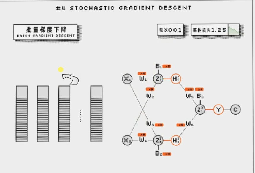批量梯度下降，计算所有节点的偏导数，然后求平均，乘上步长。更新一次参数。如果有1000个点输入，就遍历1000个点，求出各个节点的导数，求平均再乘上步长，然后更新一次参数。这个方法的缺点就是输入数据太多的话，一次迭代就需要计算很长时间。

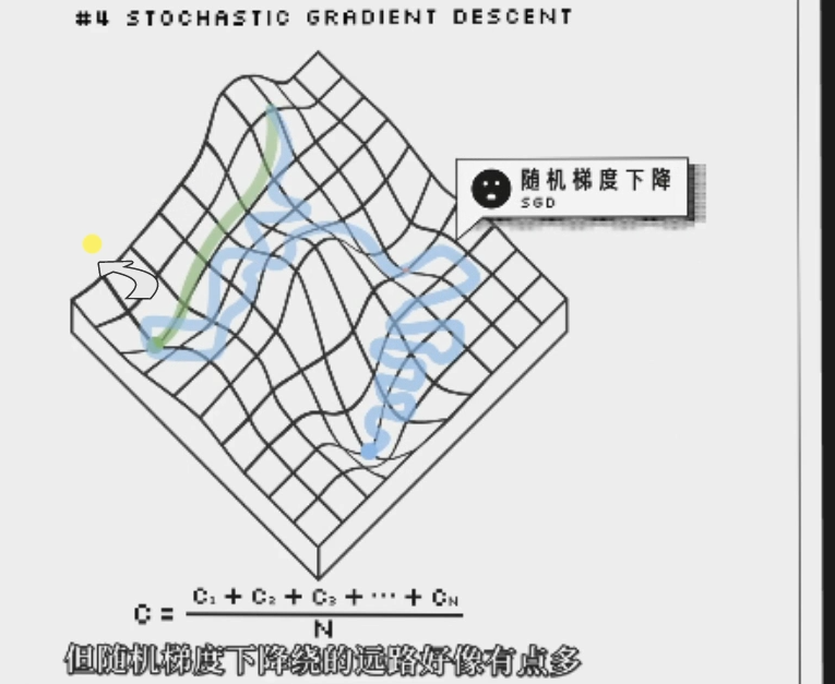
随机梯度下降

为了提高速度，因此提出了随机梯度下降。每次只针对一个样本更新参数。从输入样本数据中，随机选取一个数据，然后就更新w参数。这样虽然速度提高了，而且也能避免结果卡在局部最低点。但是这样可能找到全局最低点的效率比较慢；

小批量梯度下降

每次从输入样本中提取出一个batch出来更新参数，这个就叫做小批量梯度下降。

其他找寻最低点的方法

梯度下降找寻函数最低点是我们听的比较多的方法。其实还有很多方法去找到函数的最低点，比如SGD,Momentum,NAG,Adagrad,等等方法

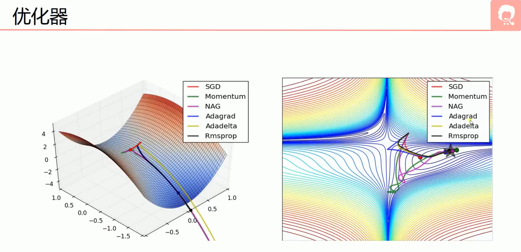
我们一般实际中，使用比较多的是SGD梯度下降法和自适应矩估计Adam优化器. 和SGD代码不同的地方就是优化器那里改一改就行了

from keras.optimizers import SGD,Adam

adam = Adam(lr=0.001) 

# 定义优化器，loss function，训练过程中计算准确率
model.compile(
    optimizer = adam,
    loss = 'categorical_crossentropy',
    metrics=['accuracy'],
)

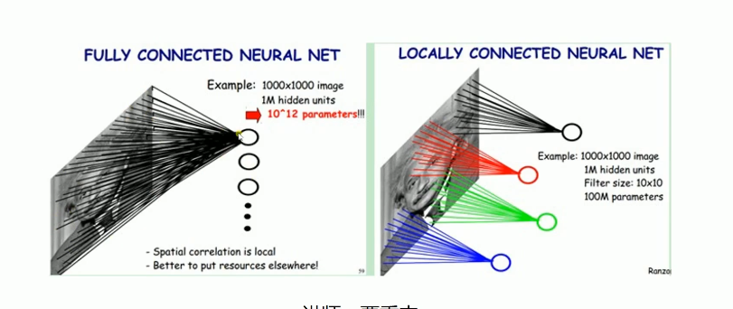
卷积神经网络

图像一般使用卷积神经网络。CNN可以通过局部感受野和权重共享减少网络参数的个数，前面的代码中，都没有出现卷积核，池化做这些操作。所以都是全链接，因此他的参数超级多，如果面对一个一层网络中，有很多节点的网络，训练起来就很慢。

基本卷积网络体验可以参考 3D visualization 可以自己去体验一下。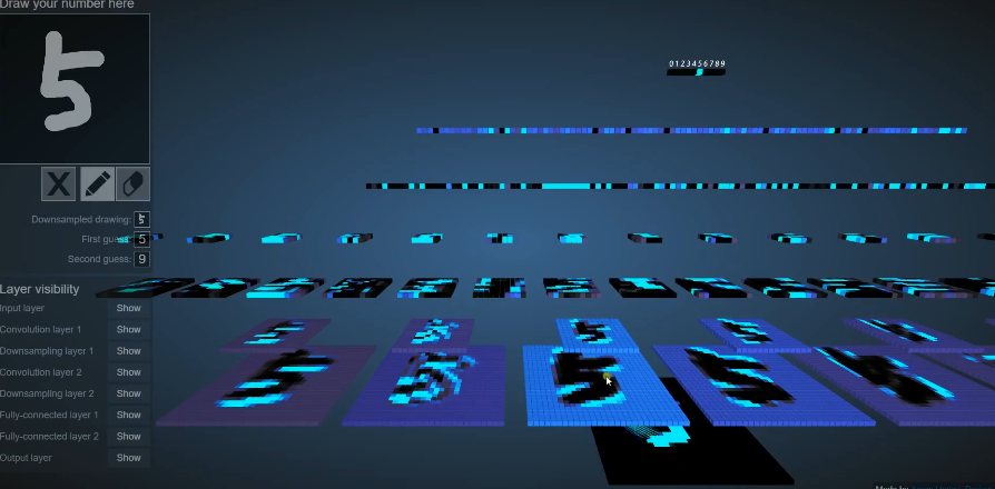

案例：CNN应用于手写数字识别

import numpy as np
from keras.datasets import mnist
from keras.utils import np_utils
from keras.models import Sequential
from keras.layers import Dense,Dropout,Convolution2D,MaxPooling2D,Flatten
from keras.optimizers import Adam

# 载入数据
(x_train,y_train),(x_test,y_test) = mnist.load_data()
# (60000,28,28)->(60000,28,28,1)  60000个数据，28*28，深度为1
x_train = x_train.reshape(-1,28,28,1)/255.0 #-1能够自动匹配，
x_test = x_test.reshape(-1,28,28,1)/255.0
# 换one hot格式
y_train = np_utils.to_categorical(y_train,num_classes=10)
y_test = np_utils.to_categorical(y_test,num_classes=10)

# 定义顺序模型
model = Sequential()

# 第一个卷积层
# input_shape 输入平面
# filters 卷积核/滤波器个数
# kernel_size 卷积窗口大小
# strides 步长
# padding padding方式 same/valid
# activation 激活函数
model.add(Convolution2D(
    input_shape = (28,28,1),
    filters = 32,
    kernel_size = 5,
    strides = 1,
    padding = 'same',
    activation = 'relu'
))
# 第一个池化层
model.add(MaxPooling2D(
    pool_size = 2,
    strides = 2,
    padding = 'same',
))
# 第二个卷积层
model.add(Convolution2D(64,5,strides=1,padding='same',activation = 'relu'))
#像64,5这样的，按照convolution2D这个函数形参顺序传入
# 第二个池化层
model.add(MaxPooling2D(2,2,'same'))
# 把第二个池化层的输出扁平化为1维
model.add(Flatten())
# 第一个全连接层
model.add(Dense(1024,activation = 'relu'))
# Dropout
model.add(Dropout(0.5))
# 第二个全连接层
model.add(Dense(10,activation='softmax'))

# 定义优化器
adam = Adam(lr=1e-4)

# 定义优化器，loss function，训练过程中计算准确率
model.compile(optimizer=adam,loss='categorical_crossentropy',metrics=['accuracy'])

# 训练模型
model.fit(x_train,y_train,batch_size=64,epochs=10)

# 评估模型
loss,accuracy = model.evaluate(x_test,y_test)

print('test loss',loss)
print('test accuracy',accuracy)

最后的识别精度：

test loss 0.02161419950425625
test accuracy 0.9929999709129333

达到了99%，而且keras这个CNN代码很有画面感，一层一层自己加上去。

RNN

如语音输入，他的输出需要关联上之前的输出，因此有了RNN，将前一次的状态当作输入，作为下一次的输入；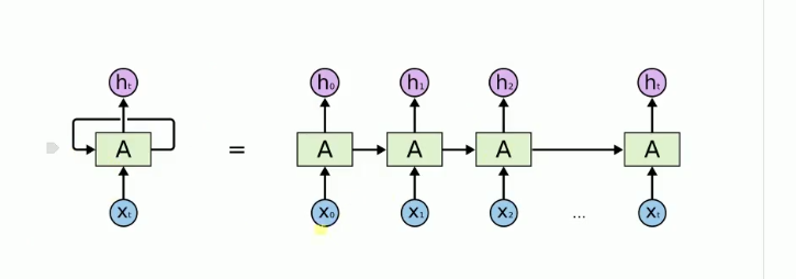

import numpy as np
from keras.datasets import mnist
from keras.utils import np_utils
from keras.models import Sequential
from keras.layers import Dense
from keras.layers.recurrent import SimpleRNN
from keras.optimizers import Adam

# 数据长度-一行有28个像素
input_size = 28
# 序列长度-一共有28行
time_steps = 28
# 隐藏层cell个数
cell_size = 50 

# 载入数据
(x_train,y_train),(x_test,y_test) = mnist.load_data()
# (60000,28,28)
x_train = x_train/255.0
x_test = x_test/255.0
# 换one hot格式
y_train = np_utils.to_categorical(y_train,num_classes=10)
y_test = np_utils.to_categorical(y_test,num_classes=10)#one hot

# 创建模型
model = Sequential()

# 循环神经网络
model.add(SimpleRNN(
    units = cell_size, # 输出
    input_shape = (time_steps,input_size), #输入
))

# 输出层
model.add(Dense(10,activation='softmax'))

# 定义优化器
adam = Adam(lr=1e-4)

# 定义优化器，loss function，训练过程中计算准确率
model.compile(optimizer=adam,loss='categorical_crossentropy',metrics=['accuracy'])

# 训练模型
model.fit(x_train,y_train,batch_size=64,epochs=10)

# 评估模型
loss,accuracy = model.evaluate(x_test,y_test)

print('test loss',loss)
print('test accuracy',accuracy)

最后输出的准确度：

test loss 0.3422239124774933
test accuracy 0.9006999731063843

这个只是例子，RNN不太适合用于分类之中，所以这里的进度并不是很高。

模型的保存和载入

保存模型

#这个导入用于保存网络结构的函数
from keras.models import model_from_json
# 在代码的最后写上
model.save('model.h5')   # HDF5文件，pip install h5py
# 只保存网络的参数
model.save_weights('my_model_weights.h5')
# 保存网络结构

json_string = model.to_json()

即可保存整个网络的模型，参数和网络结构

载入模型

#载入模型的参数和网络结构。
model = load_model('model.h5')
#只载入网络的参数
model.load_weights('my_model_weights.h5')
#载入网络结构
model = model_from_json(json_string)

绘制神经网络的结构

示例代码

import numpy as np
from keras.datasets import mnist
from keras.utils import np_utils
from keras.models import Sequential
from keras.layers import Dense,Dropout,Convolution2D,MaxPooling2D,Flatten
from keras.optimizers import Adam
from keras.utils.vis_utils import plot_model
import matplotlib.pyplot as plt 

# 载入数据
(x_train,y_train),(x_test,y_test) = mnist.load_data()
# (60000,28,28)->(60000,28,28,1)
x_train = x_train.reshape(-1,28,28,1)/255.0
x_test = x_test.reshape(-1,28,28,1)/255.0
# 换one hot格式
y_train = np_utils.to_categorical(y_train,num_classes=10)
y_test = np_utils.to_categorical(y_test,num_classes=10)

# 定义顺序模型
model = Sequential()

# 第一个卷积层
# input_shape 输入平面
# filters 卷积核/滤波器个数
# kernel_size 卷积窗口大小
# strides 步长
# padding padding方式 same/valid
# activation 激活函数
model.add(Convolution2D(
    input_shape = (28,28,1),
    filters = 32,
    kernel_size = 5,
    strides = 1,
    padding = 'same',
    activation = 'relu',
    name = 'conv1'
))
# 第一个池化层
model.add(MaxPooling2D(
    pool_size = 2,
    strides = 2,
    padding = 'same',
    name = 'pool1'
))
# 第二个卷积层
model.add(Convolution2D(64,5,strides=1,padding='same',activation = 'relu',name='conv2'))
# 第二个池化层
model.add(MaxPooling2D(2,2,'same',name='pool2'))
# 把第二个池化层的输出扁平化为1维
model.add(Flatten())
# 第一个全连接层
model.add(Dense(1024,activation = 'relu'))
# Dropout
model.add(Dropout(0.5))
# 第二个全连接层
model.add(Dense(10,activation='softmax'))

# # 定义优化器
# adam = Adam(lr=1e-4)

# # 定义优化器，loss function，训练过程中计算准确率
# model.compile(optimizer=adam,loss='categorical_crossentropy',metrics=['accuracy'])

# # 训练模型
# model.fit(x_train,y_train,batch_size=64,epochs=1)

# # 评估模型
# loss,accuracy = model.evaluate(x_test,y_test)

# print('test loss',loss)
# print('test accuracy',accuracy)

plot_model(model,to_file="model.png",show_shapes=True,show_layer_names=True,rankdir='TB') #TB表示从上到下，LR表示从左到右
plt.figure(figsize=(10,10))
img = plt.imread("model.png")
plt.imshow(img)
plt.axis('off')
plt.show()

在运行代码之前，需要先安装pydot and graphviz，我安装的时候就出现了问题。安装后也还是不能用，解决方法：画网络结构图安装了pydot和graphviz出现Failed to import pydot. You must pip install pydot and install graph错误

解决方法：

conda install graphviz
conda install pydotplus
pip install pydot

打开cmd,进入虚拟环境，按顺序安装即可。

最后在代码的目录下，会生成model.png网络结构图文件。