导航
- CVaR and VaR
- Model
- normal distribution
- student t distribution
- Case Study
- Reference
CVaR and VaR
CVaR(Conditional Value-at-Risk)也被称为Expected Shortfall(ES) 或者 Expected Tail Loss(ETL),可以解释超过给定VaR值的期望损失,在很多风险分析中,CVaR是更具有解释力,当设置了VaR阈值后,CVaR说明了在之后的 h h h天交易中的期望损失风险(即资产价值低于预先设置的VaR值). 显然VaR和资产日回报率的分布有关.
当资产回报率的尾部较厚,使用整态分布刻画是不合适的,考虑使用t分布对资产回报率分布进行描述.
Model
normal distribution
令 X X X表示 h h h日的回报率,则
V a R h , α = − x h , α VaR_{h, \alpha}=-x_{h, \alpha} VaRh,α=−xh,α
其中, P ( X < x h , α ) = α P(X<x_{h, \alpha})=\alpha P(X<xh,α)=α.
CVaR使用条件期望的形式表达
C V a R h , α ( X ) = − E ( X ∣ X < x h , α ) = − α − 1 ∫ − ∞ x h , α = x f ( x ) d x CVaR_{h, \alpha}(X)=-\mathbb{E}(X\mid X<x_{h, \alpha})=-\alpha^{-1}\int_{-\infty}^{x_{h, \alpha}}=xf(x)dx CVaRh,α(X)=−E(X∣X<xh,α)=−α−1∫−∞xh,α=xf(x)dx
对于任意连续的概率密度函数 f ( x ) f(x) f(x),需要计算 x ∼ 100 ( 1 − α ) % h x\sim 100(1-\alpha)\%h x∼100(1−α)%h天VaR的 x f ( x ) xf(x) xf(x)积分.
考虑在 X ∼ N ( μ h , σ h 2 ) X\sim N(\mu_h, \sigma_h^2) X∼N(μh,σh2)的情况下的CVaR
C V a R h , α ( X ) = α − 1 φ ( Φ − 1 ( α ) ) σ h − μ h CVaR_{h, \alpha}(X)=\alpha^{-1}\varphi(\Phi^{-1}(\alpha))\sigma_h-\mu_h CVaRh,α(X)=α−1φ(Φ−1(α))σh−μh
其中 φ ( z ) \varphi(z) φ(z)表示标准正态分布的pdf, Φ ( α ) − 1 \Phi(\alpha)^{-1} Φ(α)−1为 α \alpha α分位数.
案例:计算 h = 5 h=5 h=5的CVaR,股价年化回报率符合 σ = 41 % , μ = 0 \sigma=41\%, \mu=0 σ=41%,μ=0的正态分布,设置一年的交易日为252天计算出
σ h = σ h / 252 = 0.41 5 / 252 = 0.05798 \sigma_h=\sigma\sqrt{h/252}=0.41\sqrt{5/252}=0.05798 σh=σh/252=0.415/252=0.05798
python计算gaussian分布VaR和CVaR代码如下
import numpy as np
import matplotlib.pyplot as plt
from scipy.stats import norm
from math import sqrtdef demo_1():h, D=5, 252mu, sig = 0, 0.41muh, sigh=mu*(h/D), sig*sqrt(h/D)alpha=0.01lev=100*(1-alpha)CVaRh=alpha**(-1)*norm.pdf(norm.ppf(alpha))*sigh-muhVaRh=norm.ppf(1-alpha)*sigh-muhprint('{}% {} day Normal VaR= {:.2f}%'.format(lev, h, VaRh*100))print('{}% {} day Normal CVaR= {:.2f}%'.format(lev, h, CVaRh*100))demo_1()
student t distribution
考虑更适合肥尾的t分布进行建模,标准t分布的pdf函数为
f ν ( x ) = ( ( ν − 2 ) π ) − 1 / 2 Γ ( v 2 ) − 1 Γ ( ν + 1 2 ) ⏟ A ( 1 + ( ν − 2 ) − 1 ⏟ a x 2 ) − ( ν + 1 ) / 2 ⏟ b f_\nu(x)=\underbrace{((\nu-2)\pi)^{-1/2}\Gamma(\frac{v}{2})^{-1}\Gamma(\frac{\nu+1}{2})}_{A}(1+\underbrace{(\nu-2)^{-1}}_{a}x^2)^{\underbrace{-(\nu+1)/2}_{b}} fν(x)=A ((ν−2)π)−1/2Γ(2v)−1Γ(2ν+1)(1+a (ν−2)−1x2)b −(ν+1)/2
其中 Γ \Gamma Γ表示gamma函数, ν \nu ν表示自由度,方程一般形式为
f ν ( x ) = A ( 1 + a x 2 ) b f_\nu(x)=A(1+ax^2)^b fν(x)=A(1+ax2)b
代入到CVaR定义中得到
C V a R α , ν = − α − 1 ∫ − ∞ x α , ν x f ν ( x ) d x = − α − 1 ∫ − ∞ x α , ν x A ( 1 + a x 2 ) b d x = − A α ∫ − ∞ x α , ν x ( 1 + a x 2 ⏟ y ) b d x (1) \begin{aligned} CVaR_{\alpha, \nu}&=-\alpha^{-1}\int_{-\infty}^{x_{\alpha, \nu}}xf_\nu(x)dx\\ &=-\alpha^{-1}\int_{-\infty}^{x_{\alpha, \nu}}xA(1+ax^2)^bdx\\ &=-\frac{A}{\alpha}\int_{-\infty}^{x_{\alpha, \nu}}x(\underbrace{1+ax^2}_y)^bdx \end{aligned}\tag{1} CVaRα,ν=−α−1∫−∞xα,νxfν(x)dx=−α−1∫−∞xα,νxA(1+ax2)bdx=−αA∫−∞xα,νx(y 1+ax2)bdx(1)
令 y = 1 + a x 2 y=1+ax^2 y=1+ax2进行变换, d y = 2 a x d x , B = 1 + ( ν − 2 ) − 1 x α , ν 2 dy=2axdx,B=1+(\nu-2)^{-1}x^2_{\alpha, \nu} dy=2axdx,B=1+(ν−2)−1xα,ν2,方程 ( 1 ) (1) (1)变换得到
( 1 ) = − A α ∫ − ∞ B x ( 1 + a x 2 ) b 2 a x d y = − A 2 a α ∫ ∞ B y b d y = − A 2 a α B b + 1 b + 1 \begin{aligned} (1)&=-\frac{A}{\alpha}\int_{-\infty}^B\frac{x(1+ax^2)^b}{2ax}dy\\ &=-\frac{A}{2a\alpha}\int_{\infty}^{B}y^bdy\\ &=-\frac{A}{2a\alpha}\frac{B^{b+1}}{b+1} \end{aligned} (1)=−αA∫−∞B2axx(1+ax2)bdy=−2aαA∫∞Bybdy=−2aαAb+1Bb+1
由于 b + 1 = ( 1 − ν ) / 2 b+1=(1-\nu)/2 b+1=(1−ν)/2代入得到 ( 1 ) (1) (1)值为
− A ( ν − 2 ) − 1 α 2 B ( 1 − ν ) / 2 1 − ν -\frac{A}{(\nu-2)^{-1}\alpha}\frac{2B^{(1-\nu)/2}}{1-\nu} −(ν−2)−1αA1−ν2B(1−ν)/2
根据 f ν ( x ) f_\nu(x) fν(x)的表达式可以知道
f ν ( x ) = A B b ⇒ A = f ν ( x ) B − b = f ν ( x ) B ( 1 + ν ) / 2 f_\nu(x)=AB^b\Rightarrow A=f_\nu(x)B^{-b}=f_\nu(x)B^{(1+\nu)/2} fν(x)=ABb⇒A=fν(x)B−b=fν(x)B(1+ν)/2
代入方程 ( 1 ) (1) (1)得到CVaR值为
( 1 ) = − α − 1 f ν ( x ) B ( 1 + ν ) / 2 2 ( ν − 2 ) − 1 2 B ( 1 − ν ) / 2 1 − ν = − α − 1 f ν ( x ) ( ν − 2 ) ( 1 − ν ) − 1 B = − α − 1 ( ν − 2 ) ( 1 − ν ) − 1 ( 1 + ( ν − 2 ) − 1 x α , ν 2 ) f ν ( x α , ν ) = − α − 1 ( 1 − ν ) − 1 [ ν − 2 + x α , ν 2 ] f ν ( x α , ν ) \begin{aligned} (1)&=-\alpha^{-1}\frac{f_\nu(x)B^{(1+\nu)/2}}{2(\nu-2)^{-1}}\frac{2B^{(1-\nu)/2}}{1-\nu}\\ &=-\alpha^{-1}f_\nu(x)(\nu-2)(1-\nu)^{-1}B\\ &=-\alpha^{-1}(\nu-2)(1-\nu)^{-1}(1+(\nu-2)^{-1}x^2_{\alpha, \nu})f_\nu(x_{\alpha, \nu})\\ &=-\alpha^{-1}(1-\nu)^{-1}[\nu-2+x^2_{\alpha, \nu}]f_\nu(x_{\alpha, \nu}) \end{aligned} (1)=−α−12(ν−2)−1fν(x)B(1+ν)/21−ν2B(1−ν)/2=−α−1fν(x)(ν−2)(1−ν)−1B=−α−1(ν−2)(1−ν)−1(1+(ν−2)−1xα,ν2)fν(xα,ν)=−α−1(1−ν)−1[ν−2+xα,ν2]fν(xα,ν)
所以, h h h天,t分布下CVaR值为
C V a R h , α , ν ( X ) = − α − 1 ( 1 − ν ) − 1 [ ν − 2 + x α , ν 2 ] f ν ( x α , ν ) σ h − μ h CVaR_{h, \alpha, \nu}(X)=-\alpha^{-1}(1-\nu)^{-1}[\nu-2+x_{\alpha, \nu}^2]f_\nu(x_{\alpha, \nu})\sigma_h-\mu_h CVaRh,α,ν(X)=−α−1(1−ν)−1[ν−2+xα,ν2]fν(xα,ν)σh−μh
案例计算自由度为 6 6 6的t分布的VaR和CVaR
python计算t分布下VaR和CVaR代码如下
import numpy as np
import matplotlib.pyplot as plt
from scipy.stats import norm, t
from math import sqrtdef demo_2():h, D = 10, 252mu, sig=0, 0.41muh, sigh=mu*(h/D), sig*sqrt(h/D)alpha=0.01lev=100*(1-alpha)nu=6 # 设置自由度xanu=t.ppf(alpha, nu)CVaRh=-1/alpha*(1-nu)**(-1)*(nu-2+xanu**2)*t.pdf(xanu, nu)*sigh-muhVaRh=sqrt(h/D*(nu-2)/nu)*t.ppf(1-alpha, nu)*sig-muprint('{}% {} day t VaR= {:.2f}%'.format(lev, h, VaRh*100))print('{}% {} day t CVaR= {:.2f}%'.format(lev, h, CVaRh*100))demo_2()
可以发现,随着自由度的上升,t分布的VaR和CVaR逐渐收敛到gaussian分布的VaR和CVaR
import numpy as np
import matplotlib.pyplot as plt
from scipy.stats import norm, t
from math import sqrtdef demo_3():h, D = 10, 252mu, sig=0, 0.41muh, sigh=mu*(h/D), sig*sqrt(h/D)alpha=0.01lev=100*(1-alpha)data=[]for nu in range(5, 101):xanu=t.ppf(alpha, nu)CVaRt=-1/alpha*(1-nu)**(-1)*(nu-2+xanu**2)*t.pdf(xanu, nu)*sigh-muhVaRt=sqrt(h/D*(nu-2)/nu)*t.ppf(1-alpha, nu)*sig-muhdata.append([nu, VaRt, CVaRt])CVaRn=alpha**(-1)*norm.pdf(norm.ppf(alpha))*sigh-muhVaRn=norm.ppf(1-alpha)*sigh-muhdata=np.array(data)fig, ax=plt.subplots(figsize=(8, 6))plt.plot(data[:, 0], data[:, 1]*100, 'b-', label='VaRt')plt.plot(np.arange(5, 100), VaRn*np.ones(95)*100, 'b:', label='VaRn')plt.plot(data[:, 0], data[:, 2]*100, 'r-', label='CVaRt')plt.plot(np.arange(5, 100), CVaRn*np.ones(95)*100, 'r:', label='CVaRn')plt.xlabel('student t. d.o.f')plt.ylabel('%')plt.legend()plt.show()demo_3()

Case Study
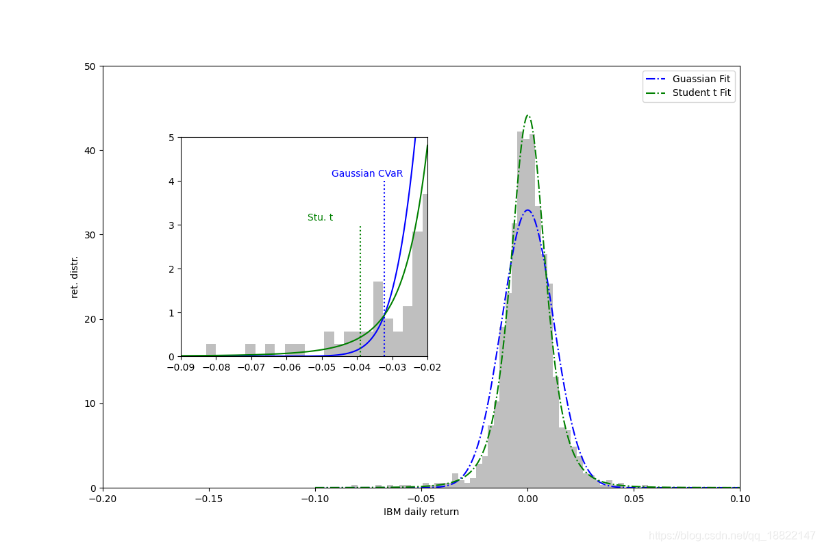
使用IBM数据进行实证分析, 使用gaussian分布和t分布拟合IBM日回报收益率得到拟合图像如下

可以发现,t分布更适合拟合这种存在高噪声的尖峰厚尾的数据,不同分布计算的CVaR和VaR值如下
99.0% 1 day gaussian VaR= 2.81%
99.0% 1 day gaussian CVaR= 3.22%
99.0% 1 day student t VaR= 2.22%
99.0% 1 day student t CVaR= 3.91%
案例python代码
import numpy as np
import matplotlib.pyplot as plt
from scipy.stats import norm, t, skew, kurtosis, kurtosistest
from math import sqrt
import pandas_datareader.data as web
import pickle# Fetching Yahoo Finance for IBM stock data
def data_fetch():data = web.DataReader('IBM', data_source='yahoo', start='2010-12-31', end='2015-12-31')['Adj Close']adj_close=np.array(data.values)ret=adj_close[1:]/adj_close[:-1]-1file=open('ibm_ret', 'wb')pickle.dump(ret, file)with open('ibm_ret', 'rb') as file:ret=pickle.load(file)dx=0.0001
x=np.arange(-0.1, 0.1, dx)# gaussian fit
mu_norm, sig_norm=norm.fit(ret)
pdf_norm=norm.pdf(x, mu_norm, sig_norm)# student t fit
nu, mu_t, sig_t=t.fit(ret)
nu=np.round(nu)
pdf_t=t.pdf(x, nu, mu_t, sig_t)# VaR and CVaR
h=1
alpha=0.01
lev=100*(1-alpha)
xanu=t.ppf(alpha, nu)CVaRn=alpha**(-1)*norm.pdf(norm.ppf(alpha))*sig_norm-mu_norm
VaRn=norm.ppf(1-alpha)*sig_norm-mu_norm
CVaRt=-1/alpha*(1-nu)**(-1)*(nu-2+xanu**2)*t.pdf(xanu, nu)*sig_t-h*mu_t
VaRt=sqrt((nu-2)/nu)*t.ppf(1-alpha, nu)*sig_t-h*mu_tprint('{}% {} day gaussian VaR= {:.2f}%'.format(lev, h, VaRn*100))
print('{}% {} day gaussian CVaR= {:.2f}%'.format(lev, h, CVaRn*100))
print('{}% {} day student t VaR= {:.2f}%'.format(lev, h, VaRt*100))
print('{}% {} day student t CVaR= {:.2f}%'.format(lev, h, CVaRt*100))plt.figure(figsize=(12, 8))
grey=0.75, 0.75, 0.75
plt.hist(ret, bins=50, density=True, color=grey, edgecolor='none')
plt.axis('tight')
plt.plot(x, pdf_norm, 'b-.', label='Guassian Fit')
plt.plot(x, pdf_t, 'g-.', label='Student t Fit')
plt.xlim([-0.2, 0.1])
plt.ylim([0, 50])
plt.legend(loc='best')
plt.xlabel('IBM daily return')
plt.ylabel('ret. distr.')# plt.savefig('ibm_fit')
# inset local
sub=plt.axes([0.22, 0.35, 0.3, 0.4])
plt.hist(ret, bins=50, density=True, color=grey, edgecolor='none')
plt.plot(x, pdf_norm, 'b')
plt.plot(x, pdf_t, 'g')
plt.plot([-CVaRt, -CVaRt], [0, 3], 'g:')
plt.plot([-CVaRn, -CVaRn], [0, 4], 'b:')
plt.text(-CVaRt-0.015, 3.1, 'Stu. t', color='g')
plt.text(-CVaRn-0.015, 4.1, 'Gaussian CVaR', color='b')
plt.xlim([-0.09, -0.02])
plt.ylim([0, 5])# plt.savefig('ibmcvar')
plt.show()
从数据和图像可以看出,Gaussian拟合计算的CVaR值存在低估风险的倾向.
Reference
CVaR Quant at risk