sunrise AI推理

旭日派中最让其期待的就是其中的BPU加速器，可以提供5TOPS的等效AI算力。

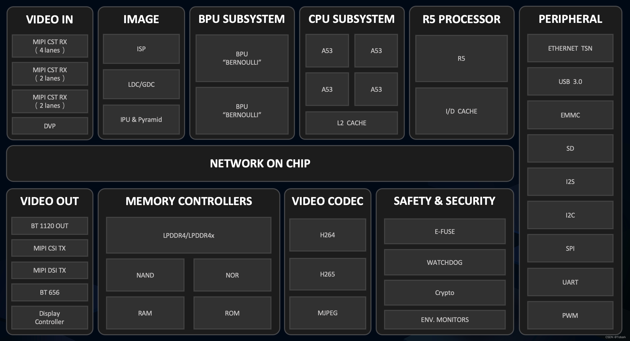
X3芯片概述

BPU是地平线自研的AI加速核，在设计过程中具体结合了AIoT/Auto的场景需求，从算法、计算架构、编译器三个方面进行了软硬协同优化，使得在功耗不变前提下提高数倍的AI计算性能。

X3和J3芯片各内置了两个伯努利2.0的BPU核，它极大提升了对先进CNN网络的支持，同时大大降低了DDR带宽占用率，可提供实时像素级视频分割和结构化视频分析等能力。

详细的内容请参考地平线芯片开发手册

1.图片分类任务

首先是系统中提供的图片分类任务样例

cd /app/ai_inference/01_basic_sample/
sudo python3 ./test_mobilenetv1.py

在test_mobilenetv1.py中对斑马的图片进行了分类，得到的结果如下，通过查看标签编号340: 'zebra'实现了对图片的准确分类。

========== Classification result ==========
cls id: 340 Confidence: 0.991851

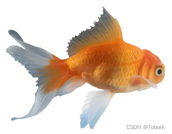
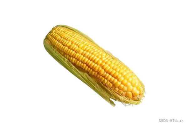
为了简单测试下分类算法的结果。使用其他图片进行测试，发现在特征明显时图片分类准确度较高，如对背景干净，特征清晰的金鱼达到了0.999884的置信度，1: 'goldfish, Carassius auratus'，也存在图片分类错误的情况存在，如对于玉米进行检测时998: 'ear, spike, capitulum'。

========== Classification result ==========
cls id: 1 Confidence: 0.999884

========== Classification result ==========
cls id: 998 Confidence: 0.753721

2.fcos目标检测快速验证

使用目标检测样例

cd /app/ai_inference/02_usb_camera_sample/
python3 usb_camera_fcos.py

在初探中已经对其进行简单展示，这里将代码进行简单分析，主要包括以下5个部分

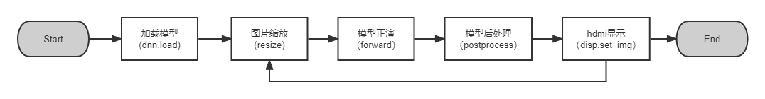
其中加载模型 和模型正演为地平线封装的模型方法，from hobot_dnn import pyeasy_dnn as dnn

hdmi显示时地平线封装的vio方法，from hobot_vio import libsrcampy as srcampy

加载的模型是通过地平线工具链编译的bin模型fcos_512x512_nv12.bin，在运行中会对输入和输出的tensor进行打印，可以看出输入的是512x512的图像信息，输入为15个tensor，其中输出包括了检测框坐标、类别、置信度得分等。

tensor type: NV12_SEPARATE
data type: uint8
layout: NCHW
shape: (1, 3, 512, 512)
15
tensor type: float32
data type: float32
layout: NHWC
shape: (1, 64, 64, 80)
tensor type: float32
data type: float32
layout: NHWC
shape: (1, 32, 32, 80)
tensor type: float32
data type: float32
layout: NHWC
shape: (1, 16, 16, 80)
tensor type: float32
data type: float32
layout: NHWC
shape: (1, 8, 8, 80)
tensor type: float32
data type: float32
layout: NHWC
shape: (1, 4, 4, 80)
tensor type: float32
data type: float32
layout: NHWC
shape: (1, 64, 64, 4)
tensor type: float32
data type: float32
layout: NHWC
shape: (1, 32, 32, 4)
tensor type: float32
data type: float32
layout: NHWC
shape: (1, 16, 16, 4)
tensor type: float32
data type: float32
layout: NHWC
shape: (1, 8, 8, 4)
tensor type: float32
data type: float32
layout: NHWC
shape: (1, 4, 4, 4)
tensor type: float32
data type: float32
layout: NHWC
shape: (1, 64, 64, 1)
tensor type: float32
data type: float32
layout: NHWC
shape: (1, 32, 32, 1)
tensor type: float32
data type: float32
layout: NHWC
shape: (1, 16, 16, 1)
tensor type: float32
data type: float32
layout: NHWC
shape: (1, 8, 8, 1)
tensor type: float32
data type: float32
layout: NHWC
shape: (1, 4, 4, 1)

3.改用yolov5进行目标检测

更换yolov5模型进行目标检测，由于工具链中提供了编译后的yolov5模型，这里可以对其直接使用，工具链相关资料在AI工具链资料包其中

horizon_xj3_open_explorer_v1.11.4_20220413\ddk\samples\ai_toolchain\model_zoo\runtime\yolov5

直接在usb_camera_fcos.py中进行模型的替换

models = dnn.load('../models/yolov5_672x672_nv12.bin')

对输入输出进行打印，可以看到输入是一个 (1, 3, 672, 672)的tensor，而输出为3层的tensor，输出的不同代表着需要对模型后处理进行重写。

tensor type: NV12_SEPARATE
data type: uint8
layout: NCHW
shape: (1, 3, 672, 672)
3
tensor type: float32
data type: float32
layout: NHWC
shape: (1, 84, 84, 255)
tensor type: float32
data type: float32
layout: NHWC
shape: (1, 42, 42, 255)
tensor type: float32
data type: float32
layout: NHWC
shape: (1, 21, 21, 255)

在这里我找到之前地平线对yolov5的后处理的相关代码和说明，这个位于\horizon_xj3_open_explorer_v1.11.4_20220413\ddk\samples\ai_toolchain\horizon_model_convert_sample\04_detection\03_yolov5\mapper

1.4 对于 YOLOv5 模型，我们在模型结构上的修改点主要在于几个输出节点处。由于目前的浮点转换工具链暂时不支持 5 维的 Reshape，所以我们在 prototxt中进行了删除，并将其移至后处理中执行。同时我们还添加了一个 transpose 算子，使该节点将以 NHWC 进行输出。这是因为在地平线芯片中， BPU 硬件本身以 NHWC 的layout 运行，这样修改后可以让 BPU 直接输出结果，而不在量化模型中引入额外的transpose。 详情请见文档中benchmark部分的图文介绍

根据说明可以看到yolov5应该属于异构量化，部分网络在后处理中执行，这也就代表需要更多的处理时间。在对于样例中给出的fcos的代码，我们主要在后处理处做出相应的调整，并将类别展示做出更换，其中主要代码也是参考了地平线中给出的yolov5的公开代码，做了部分的修改。

相关代码:

#!/usr/bin/env python3from pyexpat import model
from hobot_dnn import pyeasy_dnn as dnn
from hobot_vio import libsrcampy as srcampy
from easydict import EasyDictimport numpy as np
import cv2
import colorsys
from time import *
# detection model class namesclass_names = ["person","bicycle","car","motorcycle","airplane","bus","train","truck","boat","traffic light","fire hydrant","stop sign","parking meter","bench","bird","cat","dog","horse","sheep","cow","elephant","bear","zebra","giraffe","backpack","umbrella","handbag","tie","suitcase","frisbee","skis","snowboard","sports ball","kite","baseball bat","baseball glove","skateboard","surfboard","tennis racket","bottle",  # noqa"wine glass","cup","fork","knife","spoon","bowl","banana","apple","sandwich","orange","broccoli","carrot","hot dog","pizza","donut","cake","chair","couch","potted plant","bed","dining table","toilet","tv","laptop","mouse","remote","keyboard","cell phone","microwave","oven","toaster","sink","refrigerator","book","clock","vase","scissors","teddy bear","hair drier","toothbrush",
]
# bgr格式图片转换成 NV12格式
def bgr2nv12_opencv(image):height, width = image.shape[0], image.shape[1]area = height * widthyuv420p = cv2.cvtColor(image, cv2.COLOR_BGR2YUV_I420).reshape((area * 3 // 2,))y = yuv420p[:area]uv_planar = yuv420p[area:].reshape((2, area // 4))uv_packed = uv_planar.transpose((1, 0)).reshape((area // 2,))nv12 = np.zeros_like(yuv420p)nv12[:height * width] = ynv12[height * width:] = uv_packedreturn nv12def get_yolov5_config():yolov5_config = EasyDict()yolov5_config.ANCHORS = np.array([10, 13, 16, 30, 33, 23, 30, 61, 62, 45, 59, 119, 116, 90, 156, 198,373, 326]).reshape((3, 3, 2))yolov5_config.STRIDES = np.array([8, 16, 32])yolov5_config.NUM_CLASSES = 80yolov5_config.CLASSES = class_namesyolov5_config.INPUT_SHAPE = (672, 672)return yolov5_configdef yolov5_decoder(conv_output, num_anchors, num_classes, anchors, stride):def sigmoid(x):return 1. / (1 + np.exp(-x))# Five dimension output: [batch_size, num_anchors, output_size, output_size, 5 + num_classes]batch_size = conv_output.shape[0]output_size = conv_output.shape[-2]conv_raw_dxdy = conv_output[:, :, :, :, 0:2]conv_raw_dwdh = conv_output[:, :, :, :, 2:4]conv_raw_conf = conv_output[:, :, :, :, 4:5]conv_raw_prob = conv_output[:, :, :, :, 5:]y = np.tile(np.arange(output_size, dtype=np.int32)[:, np.newaxis],[1, output_size])x = np.tile(np.arange(output_size, dtype=np.int32)[np.newaxis, :],[output_size, 1])xy_grid = np.concatenate([x[:, :, np.newaxis], y[:, :, np.newaxis]],axis=-1)xy_grid = np.tile(xy_grid[np.newaxis, np.newaxis, :, :, :],[batch_size, num_anchors, 1, 1, 1])xy_grid = xy_grid.astype(np.float32)pred_xy = (sigmoid(conv_raw_dxdy) * 2.0 - 0.5 + xy_grid) * stridepred_wh = (sigmoid(conv_raw_dwdh) *2.0)**2 * anchors[np.newaxis, :, np.newaxis, np.newaxis, :]pred_xywh = np.concatenate([pred_xy, pred_wh], axis=-1)pred_conf = sigmoid(conv_raw_conf)pred_prob = sigmoid(conv_raw_prob)decode_output = np.concatenate([pred_xywh, pred_conf, pred_prob], axis=-1)return decode_outputdef postprocess_boxes(pred_bbox,org_img_shape,input_shape,score_threshold=0.5):"""post process boxes"""valid_scale = [0, np.inf]org_h, org_w = org_img_shapeinput_h, input_w = input_shapepred_bbox = np.array(pred_bbox)pred_xywh = pred_bbox[:, :4]pred_conf = pred_bbox[:, 4]pred_prob = pred_bbox[:, 5:]# (x, y, w, h) --> (xmin, ymin, xmax, ymax)pred_coor = np.concatenate([pred_xywh[:, :2] - pred_xywh[:, 2:] * 0.5,pred_xywh[:, :2] + pred_xywh[:, 2:] * 0.5],axis=-1)# (xmin, ymin, xmax, ymax) -> (xmin_org, ymin_org, xmax_org, ymax_org)resize_ratio = min(input_h / org_h, input_w / org_w)dw = (input_w - resize_ratio * org_w) / 2dh = (input_h - resize_ratio * org_h) / 2pred_coor[:, 0::2] = 1.0 * (pred_coor[:, 0::2] - dw) / resize_ratiopred_coor[:, 1::2] = 1.0 * (pred_coor[:, 1::2] - dh) / resize_ratio# clip the range of bboxpred_coor = np.concatenate([np.maximum(pred_coor[:, :2], [0, 0]),np.minimum(pred_coor[:, 2:], [org_w - 1, org_h - 1])],axis=-1)# drop illegal boxes whose max < mininvalid_mask = np.logical_or((pred_coor[:, 0] > pred_coor[:, 2]),(pred_coor[:, 1] > pred_coor[:, 3]))pred_coor[invalid_mask] = 0# discard invalid boxesbboxes_scale = np.sqrt(np.multiply.reduce(pred_coor[:, 2:4] - pred_coor[:, 0:2], axis=-1))scale_mask = np.logical_and((valid_scale[0] < bboxes_scale),(bboxes_scale < valid_scale[1]))# discard boxes with low scoresclasses = np.argmax(pred_prob, axis=-1)scores = pred_conf * pred_prob[np.arange(len(pred_coor)), classes]score_mask = scores > score_thresholdmask = np.logical_and(scale_mask, score_mask)coors, scores, classes = pred_coor[mask], scores[mask], classes[mask]return np.concatenate([coors, scores[:, np.newaxis], classes[:, np.newaxis]], axis=-1)def postprocess(model_output,model_hw_shape,origin_image=None,origin_img_shape=None,score_threshold=0.4,nms_threshold=0.45,dump_image=True):yolov5_config = get_yolov5_config()classes = yolov5_config.CLASSESnum_classes = yolov5_config.NUM_CLASSESanchors = yolov5_config.ANCHORSnum_anchors = anchors.shape[0]strides = yolov5_config.STRIDESinput_shape = yolov5_config.INPUT_SHAPEif origin_image is not None:org_height, org_width = origin_image.shape[1:3]else:org_height, org_width = origin_img_shapeprocess_height, process_width = model_hw_shapepred_sbbox, pred_mbbox, pred_lbbox = model_output[0].buffer.reshape([1, 84, 84, 3,85]).transpose([0, 3, 1, 2, 4]), model_output[1].buffer.reshape([1, 42, 42, 3,85]).transpose([0, 3, 1, 2, 4]), model_output[2].buffer.reshape([1, 21, 21, 3,85]).transpose([0, 3, 1, 2, 4])pred_sbbox = yolov5_decoder(pred_sbbox, num_anchors, num_classes,anchors[0], strides[0])pred_mbbox = yolov5_decoder(pred_mbbox, num_anchors, num_classes,anchors[1], strides[1])pred_lbbox = yolov5_decoder(pred_lbbox, num_anchors, num_classes,anchors[2], strides[2])pred_bbox = np.concatenate([np.reshape(pred_sbbox, (-1, 5 + num_classes)),np.reshape(pred_mbbox, (-1, 5 + num_classes)),np.reshape(pred_lbbox, (-1, 5 + num_classes))],axis=0)bboxes = postprocess_boxes(pred_bbox, (org_height, org_width),input_shape=(process_height, process_width),score_threshold=score_threshold)nms_bboxes = nms(bboxes, nms_threshold)if dump_image and origin_image is not None:print("detected item num: ", len(nms_bboxes))draw_bboxs(origin_image[0], nms_bboxes)return nms_bboxesdef get_classes(class_file_name='coco_classes.names'):'''loads class name from a file'''names = {}with open(class_file_name, 'r') as data:for ID, name in enumerate(data):names[ID] = name.strip('\n')return namesdef draw_bboxs(image, bboxes, gt_classes_index=None, classes=get_classes()):"""draw the bboxes in the original image"""num_classes = len(classes)image_h, image_w, channel = image.shapehsv_tuples = [(1.0 * x / num_classes, 1., 1.) for x in range(num_classes)]colors = list(map(lambda x: colorsys.hsv_to_rgb(*x), hsv_tuples))colors = list(map(lambda x: (int(x[0] * 255), int(x[1] * 255), int(x[2] * 255)),colors))fontScale = 0.5bbox_thick = int(0.6 * (image_h + image_w) / 600)for i, bbox in enumerate(bboxes):coor = np.array(bbox[:4], dtype=np.int32)if gt_classes_index == None:class_index = int(bbox[5])score = bbox[4]else:class_index = gt_classes_index[i]score = 1bbox_color = colors[class_index]c1, c2 = (coor[0], coor[1]), (coor[2], coor[3])cv2.rectangle(image, c1, c2, bbox_color, bbox_thick)classes_name = classes[class_index]bbox_mess = '%s: %.2f' % (classes_name, score)t_size = cv2.getTextSize(bbox_mess,0,fontScale,thickness=bbox_thick // 2)[0]cv2.rectangle(image, c1, (c1[0] + t_size[0], c1[1] - t_size[1] - 3),bbox_color, -1)cv2.putText(image,bbox_mess, (c1[0], c1[1] - 2),cv2.FONT_HERSHEY_SIMPLEX,fontScale, (0, 0, 0),bbox_thick // 2,lineType=cv2.LINE_AA)print("{} is in the picture with confidence:{:.4f}".format(classes_name, score))#    cv2.imwrite("demo.jpg", image)return imagedef yolov5_decoder(conv_output, num_anchors, num_classes, anchors, stride):def sigmoid(x):return 1. / (1 + np.exp(-x))# Five dimension output: [batch_size, num_anchors, output_size, output_size, 5 + num_classes]batch_size = conv_output.shape[0]output_size = conv_output.shape[-2]conv_raw_dxdy = conv_output[:, :, :, :, 0:2]conv_raw_dwdh = conv_output[:, :, :, :, 2:4]conv_raw_conf = conv_output[:, :, :, :, 4:5]conv_raw_prob = conv_output[:, :, :, :, 5:]y = np.tile(np.arange(output_size, dtype=np.int32)[:, np.newaxis],[1, output_size])x = np.tile(np.arange(output_size, dtype=np.int32)[np.newaxis, :],[output_size, 1])xy_grid = np.concatenate([x[:, :, np.newaxis], y[:, :, np.newaxis]],axis=-1)xy_grid = np.tile(xy_grid[np.newaxis, np.newaxis, :, :, :],[batch_size, num_anchors, 1, 1, 1])xy_grid = xy_grid.astype(np.float32)pred_xy = (sigmoid(conv_raw_dxdy) * 2.0 - 0.5 + xy_grid) * stridepred_wh = (sigmoid(conv_raw_dwdh) *2.0)**2 * anchors[np.newaxis, :, np.newaxis, np.newaxis, :]pred_xywh = np.concatenate([pred_xy, pred_wh], axis=-1)pred_conf = sigmoid(conv_raw_conf)pred_prob = sigmoid(conv_raw_prob)decode_output = np.concatenate([pred_xywh, pred_conf, pred_prob], axis=-1)return decode_outputdef nms(bboxes, iou_threshold, sigma=0.3, method='nms'):def bboxes_iou(boxes1, boxes2):boxes1 = np.array(boxes1)boxes2 = np.array(boxes2)boxes1_area = (boxes1[..., 2] - boxes1[..., 0]) * \(boxes1[..., 3] - boxes1[..., 1])boxes2_area = (boxes2[..., 2] - boxes2[..., 0]) * \(boxes2[..., 3] - boxes2[..., 1])left_up = np.maximum(boxes1[..., :2], boxes2[..., :2])right_down = np.minimum(boxes1[..., 2:], boxes2[..., 2:])inter_section = np.maximum(right_down - left_up, 0.0)inter_area = inter_section[..., 0] * inter_section[..., 1]union_area = boxes1_area + boxes2_area - inter_areaious = np.maximum(1.0 * inter_area / union_area,np.finfo(np.float32).eps)return iousclasses_in_img = list(set(bboxes[:, 5]))best_bboxes = []for cls in classes_in_img:cls_mask = (bboxes[:, 5] == cls)cls_bboxes = bboxes[cls_mask]while len(cls_bboxes) > 0:max_ind = np.argmax(cls_bboxes[:, 4])best_bbox = cls_bboxes[max_ind]best_bboxes.append(best_bbox)cls_bboxes = np.concatenate([cls_bboxes[:max_ind], cls_bboxes[max_ind + 1:]])iou = bboxes_iou(best_bbox[np.newaxis, :4], cls_bboxes[:, :4])weight = np.ones((len(iou),), dtype=np.float32)assert method in ['nms', 'soft-nms']if method == 'nms':iou_mask = iou > iou_thresholdweight[iou_mask] = 0.0if method == 'soft-nms':weight = np.exp(-(1.0 * iou ** 2 / sigma))cls_bboxes[:, 4] = cls_bboxes[:, 4] * weightscore_mask = cls_bboxes[:, 4] > 0.cls_bboxes = cls_bboxes[score_mask]return best_bboxesdef print_properties(pro):print("tensor type:", pro.tensor_type)print("data type:", pro.dtype)print("layout:", pro.layout)print("shape:", pro.shape)if __name__ == '__main__':models = dnn.load('../models/yolov5_672x672_nv12.bin')# 打印输入 tensor 的属性print_properties(models[0].inputs[0].properties)# 打印输出 tensor 的属性print(len(models[0].outputs))for output in models[0].outputs:print_properties(output.properties)# 打开 usb camera: /dev/video8cap = cv2.VideoCapture(8)if(not cap.isOpened()):exit(-1)print("Open usb camera successfully")# 设置usb camera的输出图像格式为 MJPEG， 分辨率 1920 x 1080codec = cv2.VideoWriter_fourcc( 'M', 'J', 'P', 'G' )cap.set(cv2.CAP_PROP_FOURCC, codec)cap.set(cv2.CAP_PROP_FPS, 30)cap.set(cv2.CAP_PROP_FRAME_WIDTH, 1920)cap.set(cv2.CAP_PROP_FRAME_HEIGHT, 1080)# Get HDMI display objectdisp = srcampy.Display()# For the meaning of parameters, please refer to the relevant documents of HDMI displaydisp.display(0, 1920, 1080)while True:begin_time = time()_ ,frame = cap.read()# print(frame.shape)if frame is None:print("Failed to get image from usb camera")# 把图片缩放到模型的输入尺寸# 获取算法模型的输入tensor 的尺寸h, w = models[0].inputs[0].properties.shape[2], models[0].inputs[0].properties.shape[3]des_dim = (w, h)resized_data = cv2.resize(frame, des_dim, interpolation=cv2.INTER_AREA)nv12_data = bgr2nv12_opencv(resized_data)cv_time = time()print("cv_time         = ",cv_time-begin_time)# Forwardoutputs = models[0].forward(nv12_data)Forward_time = time()print("Forward_time    = ",Forward_time-cv_time)# Do post processinput_shape = (h, w)prediction_bbox = postprocess(outputs, input_shape, origin_img_shape=(1080,1920))postprocess_time = time()print("postprocess_time= ",postprocess_time-Forward_time)# Draw bboxsbox_bgr = draw_bboxs(frame, prediction_bbox)cv2.imwrite("imf.jpg", box_bgr)# Convert to nv12 for HDMI displaybox_nv12 = bgr2nv12_opencv(box_bgr)disp.set_img(box_nv12.tobytes())end_time = time()runtime = end_time -begin_timeprint('time:',runtime)

检测结果：

运行指令

python3 usb_camera_yolov5.py 

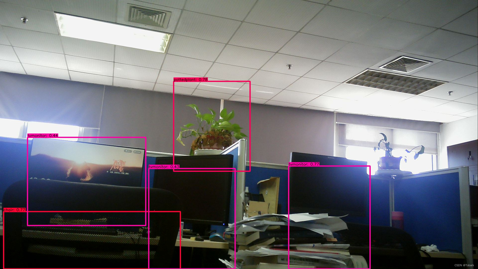
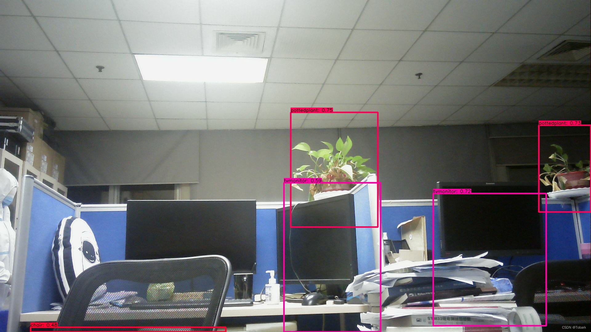
将检测结果输出，可以看到对环境中的大部分物品做出了及时的检测，置信度也很高。

对时间进行统计，检测的时间根据实际环境中的复杂度变化而变化，经过实际测试发现在0.5s~0.8s之间，检测结果较快。主要对cv_time（获取图像并缩放到模型的输入尺寸）、forward_time（模型的正向推演）、postprocess_time（后处理）时间进行了统计，其中模型量化后的时间主要是Forward_time，可以看到需要的时间较短，表明模型的量化有效的减少了检测时间。占用的时间主要集中在后处理和显示，还有优化的空间。

time: 0.8004379272460938
cv_time         =  0.15749073028564453
Forward_time    =  0.06625533103942871
postprocess_time=  0.38094043731689453
chair is in the picture with confidence:0.8259
pottedplant is in the picture with confidence:0.7951
tvmonitor is in the picture with confidence:0.7798
tvmonitor is in the picture with confidence:0.4708
tvmonitor is in the picture with confidence:0.4420
time: 0.8241267204284668
cv_time         =  0.1624467372894287
Forward_time    =  0.06629300117492676
postprocess_time=  0.3649098873138428
chair is in the picture with confidence:0.6791
pottedplant is in the picture with confidence:0.7784
tvmonitor is in the picture with confidence:0.7809
tvmonitor is in the picture with confidence:0.5400

4.使用工具链量化模型

查看工具链介绍主要有以下两种方式：

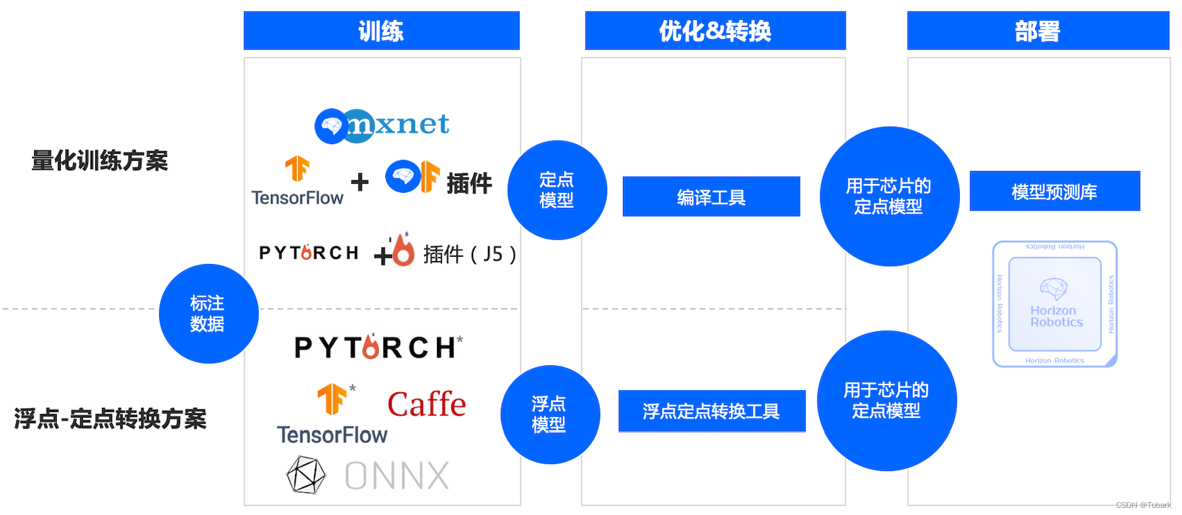
这里使用浮点转定点工具链，这种方法适用于最多的模型，详细介绍可以去查看数据链的视频。

使用wegt下在docker文件，安装docker读取镜像

docker image ls
docker run -it hub.hobot.cc/aitools/ai_toolchain_centos_7_xj3:v2.1.7 /bin/bash

这里发现其中又yolov5s的相关内容，使用该模型进行快速部署

cd /open_explorer/horizon_xj3_open_explorer_v2.1.7_20220520/ddk/samples/ai_toolchain/horizon_model_convert_sample/04_detection/03_yolov5s/mapper
bash 01_check.sh
bash 02_preprocess.sh
bash 03_build.sh   #此步骤需要耗费一定时间

在model_output中输出了yolov5s_672x672_nv12.bin ，由于输出模型一致，直接在板子代码中修改运行，得到了与yolo相似的效果。

5.最后

非常有幸作为板子的测试者，第一次使用带有AI加速功能的板子，AI加速还是有惊喜，模型量化后大大减少了CPU的压力，实际测试帧率还有较快。由于教程比较清晰简单，上手也没有难度，很快有了结果，同时有丰富的程序案例，也给了我们自己创作的空间。因为两个帖子主要对板子的一些功能进行了简单测试，笔者水平较低，不一定代表了板子的真实性能，可能会被大家较先看到，后面还有更多大佬的丰富的分享，这里只是抛砖引玉一下，大家可以期待一波。