文章目录
- 声明
- 一、问题描述
- 二、编程实现
- 1.加载数据集
- 2.使用mini-batch
- 3.利用pytorch搭建神经网络
- 3.1 利用torch.nn简单封装模型
- 3.2 定义优化算法和损失函数
- 4.整体代码
声明
本博客只是记录一下本人在深度学习过程中的学习笔记和编程经验,大部分代码是参考了【中文】【吴恩达课后编程作业】Course 2 - 改善深层神经网络 - 第三周作业这篇博客,对其代码实现了复现,但是原博客中代码使用的是tensorflow,而我在学习生活中主要用到的是pytorch,所以此次作业我使用pytorch框架来完成。因此,代码或文字表述中还存在一些问题,请见谅,之前的博客也是主要参考这个大佬。下文中的完整代码已经上传到百度网盘中,提取码:gp3h。
所以开始作业前,请大家安装好pytorch的环境,我代码是在服务器上利用gpu加速运行的,但是cpu版本的pytorch也能运行,只是速度会比较慢。
一、问题描述
这周作业的任务是利用softmax层完成一个多分类问题,利用神经网络识别图片中手指比划的数字,大致如下:

二、编程实现
1.加载数据集
用matplotlib绘制数据集中的数据,可以查看图片:
from tf_utils import load_dataset
import matplotlib.pyplot as pltX_train_orig , Y_train_orig , X_test_orig , Y_test_orig , classes = load_dataset()index = 12
plt.imshow(X_train_orig[index])
plt.show()
图片如下:
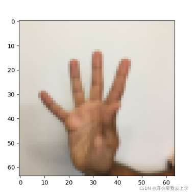
通过上述代码,我们得到的X_train_orig的维度为(1080,64,64,3),在之前的作业中我们知道,(64,64,3)表示的是一张图片的信息,而1080表示训练集中的样本数量。
def data_processing():X_train_orig, Y_train_orig, X_test_orig, Y_test_orig, classes = load_dataset()X_train_flatten = X_train_orig.reshape(X_train_orig.shape[0], -1).T / 255X_test_flatten = X_test_orig.reshape(X_test_orig.shape[0], -1).T / 255return X_train_flatten, Y_train_orig, X_test_flatten, Y_test_orig, classes
数据处理后训练集中的维度变为(12288,1080),其中12288=64x64x3,而标签集的维度在下文中细说。
2.使用mini-batch
在之前的编程作业中已经对mini-batch的使用有了较为全面的了解,而且mini-batch并不是本次作业的重点,在这里就贴出划分mini-batch的代码,不再做进一步解释:
def random_mini_batches(X, Y, mini_batch_size=64, seed=0):"""Creates a list of random minibatches from (X, Y)Arguments:X -- input data, of shape (input size, number of examples)Y -- true "label" vector (containing 0 if cat, 1 if non-cat), of shape (1, number of examples)mini_batch_size - size of the mini-batches, integerseed -- this is only for the purpose of grading, so that you're "random minibatches are the same as ours.Returns:mini_batches -- list of synchronous (mini_batch_X, mini_batch_Y)"""m = X.shape[1] # number of training examplesmini_batches = []np.random.seed(seed)# Step 1: Shuffle (X, Y)permutation = list(np.random.permutation(m))shuffled_X = X[:, permutation]shuffled_Y = Y[:, permutation].reshape((Y.shape[0], m))# Step 2: Partition (shuffled_X, shuffled_Y). Minus the end case.num_complete_minibatches = math.floor(m / mini_batch_size) # number of mini batches of size mini_batch_size in your partitionningfor k in range(0, num_complete_minibatches):mini_batch_X = shuffled_X[:, k * mini_batch_size: k * mini_batch_size + mini_batch_size]mini_batch_Y = shuffled_Y[:, k * mini_batch_size: k * mini_batch_size + mini_batch_size]mini_batch = (mini_batch_X, mini_batch_Y)mini_batches.append(mini_batch)# Handling the end case (last mini-batch < mini_batch_size)if m % mini_batch_size != 0:mini_batch_X = shuffled_X[:, num_complete_minibatches * mini_batch_size: m]mini_batch_Y = shuffled_Y[:, num_complete_minibatches * mini_batch_size: m]mini_batch = (mini_batch_X, mini_batch_Y)mini_batches.append(mini_batch)return mini_batches
3.利用pytorch搭建神经网络
我们需要搭建的神经网络结构为:LINEAR -> RELU -> LINEAR -> RELU -> LINEAR -> SOFTMAX。可以看出,与之前相比只是把输出层的激活函数换成softmax函数,随之而变的是输出层的神经元个数,因为是六分类,对应的神经元个数为6。
3.1 利用torch.nn简单封装模型
class Model(torch.nn.Module):def __init__(self, N_in, h1, h2, D_out):super(Model, self).__init__()self.linear1 = torch.nn.Linear(N_in, h1)self.relu1 = torch.nn.ReLU()self.linear2 = torch.nn.Linear(h1, h2)self.relu2 = torch.nn.ReLU()self.linear3 = torch.nn.Linear(h2, D_out)self.model = torch.nn.Sequential(self.linear1, self.relu1, self.linear2, self.relu2, self.linear3)def forward(self, x):return self.model(x)
根据题目要求定义需要的计算层,并作为参数依次传入 Sequential 函数内,传入顺序决定了计算顺序,千万不能弄错。
定义一个前向传播的函数,可以看出,利用pytorch做前向传播极大的减少了代码量。
3.2 定义优化算法和损失函数
optimizer = torch.optim.Adam(m.model.parameters(), lr=learning_rate)
loss_fn = torch.nn.CrossEntropyLoss()
优化算法这里采用的是Adam优化算法,直接使用torch.optim包里面的函数即可,记住需要把神经网络的参数还有定义的学习率传入到函数里面。
损失函数这里使用的是交叉熵函数,关于交叉熵背后的数学原理相信大家已经在视频中有了大致了解,在这里就不再做过多解释,但是使用pytorch封装好的交叉熵函数时需要注意参数的传入。
通过前向传播,我们得到输出层的结果为(n,6),这里的n表示的时输入的样本数量,而每一列的6个数据表示的是样本属于六个类别的概率,这应该很好理解。
计算损失时,我们需要将预测标签值y_pred和实际标签值y传入损失函数中,y_pred的维度为(n,6),而y的维度为(n,),没错,我们要将样本的实际标签值设置成1维,交叉熵函数会在内部将y转换为one-hot形式,y的维度会变成(n,6)。而在tensorflow框架中,损失函数不会帮我们完成one-hot的转换,我们要自己完成。
还有一点需要指出,CrossEntropyLoss 在内部完成了softmax的功能,所以不需要在前向传播的过程中定义softmax计算层。
4.整体代码
import torchnum = torch.cuda.device_count()
device = torch.device("cuda:0" if torch.cuda.is_available() else "cpu")from tf_utils import load_dataset, random_mini_batches, convert_to_one_hot
from model import Modeldef data_processing():X_train_orig, Y_train_orig, X_test_orig, Y_test_orig, classes = load_dataset()X_train_flatten = X_train_orig.reshape(X_train_orig.shape[0], -1).T / 255X_test_flatten = X_test_orig.reshape(X_test_orig.shape[0], -1).T / 255return X_train_flatten, Y_train_orig, X_test_flatten, Y_test_orig, classesif __name__ == "__main__":X_train_flatten, Y_train, X_test_flatten, Y_test, classes = data_processing()X_train_flatten = torch.from_numpy(X_train_flatten).to(torch.float32).to(device)Y_train = torch.from_numpy(Y_train).to(torch.float32).to(device)X_test_flatten = torch.from_numpy(X_test_flatten).to(torch.float32).to(device)Y_test = torch.from_numpy(Y_test).to(torch.float32).to(device)D_in, h1, h2, D_out = 12288, 25, 12, 6m = Model(D_in, h1, h2, D_out)m.to(device)epoch_num = 1500learning_rate = 0.0001minibatch_size = 32seed = 3costs = []optimizer = torch.optim.Adam(m.model.parameters(), lr=learning_rate)loss_fn = torch.nn.CrossEntropyLoss()for epoch in range(epoch_num):epoch_cost = 0num_minibatches = int(X_train_flatten.size()[1] / minibatch_size)minibatches = random_mini_batches(X_train_flatten, Y_train, minibatch_size, seed)for minibatch in minibatches:(minibatch_X, minibatch_Y) = minibatchy_pred = m.forward(minibatch_X.T)y = minibatch_Y.Ty = y.view(-1)loss = loss_fn(y_pred, y.long())epoch_cost = epoch_cost + loss.item()optimizer.zero_grad()loss.backward()optimizer.step()epoch_cost = epoch_cost / (num_minibatches + 1)if epoch % 5 == 0:costs.append(epoch_cost)# 是否打印:if epoch % 100 == 0:print("epoch = " + str(epoch) + "    epoch_cost = " + str(epoch_cost))
损失函数计算结果:
epoch = 0    epoch_cost = 1.8013256788253784
epoch = 100    epoch_cost = 0.8971561684327967
epoch = 200    epoch_cost = 0.6031410886960871
epoch = 300    epoch_cost = 0.396172211450689
epoch = 400    epoch_cost = 0.2640543882461155
epoch = 500    epoch_cost = 0.17116783581235828
epoch = 600    epoch_cost = 0.10572761395836577
epoch = 700    epoch_cost = 0.060585571726893675
epoch = 800    epoch_cost = 0.03220567786518265
epoch = 900    epoch_cost = 0.01613416599438471
epoch = 1000    epoch_cost = 0.007416377563084311
epoch = 1100    epoch_cost = 0.0030659845283748034
epoch = 1200    epoch_cost = 0.0027029767036711905
epoch = 1300    epoch_cost = 0.0013640667637125315
epoch = 1400    epoch_cost = 0.0005838543190346921