---

前言

关于$OpenDRIVE$的相关内容请查看这篇博客：一文读懂opendrive的xodr文件内容

---

我这篇的内容主要是将其中的数据可视化，采用数形结合的方式帮助自己更好地理解$OpenDRIVE$中的单个元素。把单个元素理解清楚了，后期就可以把单个元素组合起来，画出整个地图，前期会用$matlab$写一写，等单个元素理解清楚了后期会用$python$来处理$.xodr$文件。

一、$planView$

$planView$下的元素是地图中最重要的参考线，参考线中主要有三类曲线，直线、螺旋线、弧线和含参的三次曲线。

参数三次曲线

在此用一段三次曲线的例子来说明，例子如下:

s1="0.000000000000e+00"; x1="-2.855056647744e+03" ;y1="5.163670291832e+03"; hdg1="3.678546924447e-02"; length1="2.500078567784e+01";
aU1="0.000000000000e+00"; bU1="2.500000000001e+01" ;cU1="-1.179775702581e-02" ;dU1="5.898878510380e-03"; aV1="0.000000000000e+00"; bV1="0.000000000000e+00" ;cV1="1.086110728936e+00"; dV1="-5.430553643517e-01" ;pRange1=1;s2="2.500078567784e+01"; x2="-2.830099427400e+03"; y2="5.165132192211e+03" ;hdg2="5.850939248778e-02" ;length2="2.500000000004e+01";
aU2="0.000000000000e+00"; bU2="2.500000000004e+01" ;cU2="-2.433465986771e-14"; dU2="1.625209696867e-14" ;aV2="0.000000000000e+00" ;bV2="2.220446049250e-16"; cV2="6.938933641603e-10" ;dV2="-4.614609867787e-10"; pRange2=1;s3="5.000078567788e+01" ;x3="-2.805142207057e+03" ;y3="5.166594092591e+03" ;hdg3="5.850939248792e-02"; length3="2.499999999990e+01";
aU3="0.000000000000e+00"; bU3="2.499999999990e+01" ;cU3="1.028584409687e-15"; dU3="0.000000000000e+00" ;aV3="0.000000000000e+00"; bV3="0.000000000000e+00"; cV3="-5.225974468605e-10" ;dV3="2.935688096311e-10" ;pRange3=1;s4="7.500078567777e+01"; x4="-2.780184986713e+03"; y4="5.168055992971e+03"; hdg4="5.850939248134e-02"; length4="3.259185499839e+01";
aU4="0.000000000000e+00" ;bU4="3.259077023178e+01" ;cU4="8.141001992985e-03"; dU4="-8.141001992975e-03"; aV4="0.000000000000e+00" ;bV4="2.220446049250e-16"; cV4="-7.284070115927e-01" ;dV4="7.284070116768e-01" ;pRange4=1;

该参考线由四段三次曲线组成，利用matlab代码将其合成一段曲线，代码如下：

s1=double(s1);
s2=double(s2);
s3=double(s3);
s4=double(s4);x1=double(x1);
x2=double(x2);
x3=double(x3);
x4=double(x4);
y1=double(y1);
y2=double(y2);
y3=double(y3);
y4=double(y4);
hdg1=double(hdg1);
hdg2=double(hdg2);
hdg3=double(hdg3);
hdg4=double(hdg4);
length1=double(length1);
length2=double(length2);
length3=double(length3);
length4=double(length4);aU1=double(aU1);
aU2=double(aU2);
aU3=double(aU3);
aU4=double(aU4);
bU1=double(bU1);
bU2=double(bU2);
bU3=double(bU3);
bU4=double(bU4);
cU1=double(cU1);
cU2=double(cU2);
cU3=double(cU3);
cU4=double(cU4);
dU1=double(dU1);
dU2=double(dU2);
dU3=double(dU3);
dU4=double(dU4);aV1=double(aV1);
aV2=double(aV2);
aV3=double(aV3);
aV4=double(aV4);
bV1=double(bV1);
bV2=double(bV2);
bV3=double(bV3);
bV4=double(bV4);
cV1=double(cV1);
cV2=double(cV2);
cV3=double(cV3);
cV4=double(cV4);
dV1=double(dV1);
dV2=double(dV2);
dV3=double(dV3);
dV4=double(dV4);
uv1=zeros(101,2);
index1=0;
for i1=0:0.01:1u1=aU1+bU1*i1+cU1*i1.^2+dU1*i1.^3;v1=aV1+bV1*i1+cV1*i1.^2+dV1*i1.^3;index1=index1+1;[ X1,Y1]=Coordinate_rotation(u1,v1,hdg1);%u、v是局部坐标值，为了将其转换到全局坐标需要一次旋转和平移，这里是旋转一次，调用的函数Coordinate_rotation在后面有写；X1=x1+X1;%x值平移；Y1=Y1+y1;%y值平移，后面不再重复；uv1(index1,1)=X1;uv1(index1,2)=Y1;
end
figure(1)
plot(uv1(:,1),uv1(:,2))uv2=zeros(101,2);
index2=0;
for i2=0:0.01:1u2=aU2+bU2*i2+cU2*i2.^2+dU2*i2.^3;v2=aV2+bV2*i2+cV2*i2.^2+dV2*i2.^3;index2=index2+1;[ X2,Y2]=Coordinate_rotation(u2,v2,hdg2);X2=x2+X2;Y2=Y2+y2;uv2(index2,1)=X2;uv2(index2,2)=Y2;
end
figure(2)
plot(uv2(:,1),uv2(:,2))uv3=zeros(101,2);
index3=0;
for i3=0:0.01:1u3=aU3+bU3*i3+cU3*i3.^2+dU3*i3.^3;v3=aV3+bV3*i3+cV3*i3.^2+dV3*i3.^3;index3=index3+1;[ X3,Y3]=Coordinate_rotation(u3,v3,hdg3);X3=x3+X3;Y3=Y3+y3;uv3(index3,1)=X3;uv3(index3,2)=Y3;
end
figure(3)
plot(uv3(:,1),uv3(:,2))uv4=zeros(101,2);
index4=0;
for i4=0:0.01:1u4=aU4+bU4*i4+cU4*i4.^2+dU4*i4.^3;v4=aV4+bV4*i4+cV4*i4.^2+dV4*i4.^3;index4=index4+1;[ X4,Y4]=Coordinate_rotation(u4,v4,hdg4);X4=x4+X4;Y4=Y4+y4;uv4(index4,1)=X4;uv4(index4,2)=Y4;
end
figure(4)
plot(uv4(:,1),uv4(:,2))
point=zeros(404,2);
for j=1:101point(j,1)=uv1(j,1);point(j,2)=uv1(j,2);point(j+101,1)=uv2(j,1);point(j+101,2)=uv2(j,2);point(j+101*2,1)=uv3(j,1);point(j+101*2,2)=uv3(j,2);point(j+101*3,1)=uv4(j,1);point(j+101*3,2)=uv4(j,2);
end
figure(5)
plot(point(:,1),point(:,2))

function [x,y] = Coordinate_rotation(X,Y,theta)%X、Y是局部坐标值，theta对应于hdg角度,x、y全局坐标值。
x=X*cos(theta)-Y*sin(theta);
y=X*sin(theta)+Y*cos(theta);
end

生成的四段曲线分别如下，分别对应$figure1$,$figure2$,$figure3$,$figure4$，这里的横纵坐标就是全局坐标系下的$x、y$：



最终合成一段曲线figure5如下：

弧线

直线就不说了，在做弧线时，注意曲率的正负，决定了是右曲线还是左曲线，以下这个例子曲率为正，那么就是左曲线，从起点处$x=278,y=-828$逆时针画圆弧，可以看出圆弧完全位于起点的左边，若曲率为负，就和例子相反了，示例如下：

clear all
clc
% %%
% <planView>
%     <geometry x="278" y="-828" hdg="0.50" s="0" length="34">
%         <arc curvature="0.06"/>
%     </geometry>
% </planView>
% %%
x_arc=278 ;y_arc=-828;hdg_arc=0.50; s_arc=0 ;length_arc=34;
curvature=0.06;
r_arc=1/curvature;
xc=x_arc-r_arc*sin(hdg_arc);
yc=y_arc+r_arc*cos(hdg_arc);
theta=length_arc/r_arc;
angle_start=pi/2-hdg_arc;
angle_end=theta+pi/2-hdg_arc;
t=-angle_start:0.01:angle_end;
x=xc+r_arc* cos(t);
y= yc+r_arc*sin(t);
plot(x,y);

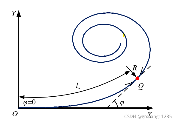
螺旋线

直线和弧线的连接需要用到螺旋线，曲线的曲率从$0$（直线）开始随着曲线的长度线性增加，直至最大值（弧线），这里的螺旋线为欧拉螺旋线，欧拉螺线（$Eulerspiral$）/ 羊角螺线（$clothoid$）的特性是它的曲率随着它的曲线长度线性地改变，因为它的这个性质，该曲线存在于很多地方，在$PreScan$中的道路元素里就有它，比如过山车 、公路的连接都会用到它，这个曲线不好画，参数方程如下：$$\{\begin{array}{c}x=C(t)\\ y=S(t)\end{array}$$
其中$C(t)$, $S(t)$ 是 菲涅耳积分 ($Fresnelintegral$)
$$\{\begin{array}{cc}C(x)& ={\int }_0^{x}cos(t^2)\mathrm{d}t={\sum }_{n=0}^{\infty }(-1{)}^n\frac{x^{4n+1}}{(4n+1)(2n)！}\\ S(x)& ={\int }_0^{x}sin(t^2)\mathrm{d}t={\sum }_{n=0}^{\infty }(-1{)}^n\frac{x^{4n+3}}{(4n+3)(2n+1)！}\end{array}$$
在$OpenDRIVE$示例如下：

% curvStart="0.0" ;curvEnd="0.013";
% s="100.0" ;x="38.00"; y="-1.81" ;hdg="0.33" ;length="30.00";

画图的$Matlab$代码如下,没有做旋转和平移，自行实践：

ls=0:0.001:0.1950;
len_ls=length(ls);
syms t;
c1=(1/sqrt(2*pi))*(cos(t)/sqrt(t));
s1=(1/sqrt(2*pi))*(sin(t)/sqrt(t));
xy=zeros(len_ls,2);
ccc=sqrt(pi*30/0.013);
for i=1:len_lsC_ls=int(c1,0,ls(1,i));S_ls=int(s1,0,ls(1,i));xy(i,1)=ccc*C_ls;xy(i,2)=ccc*S_ls;
end
plot(xy(:,1),xy(:,2))

画图的原理如下：

二、$elevationProfile$

在$OpenDRIVE$中，在纵向上，高程$Roadelevation$用 $elevationProfile$ 元素中的 $elevation$ 元素来表示。从图中可以看到两段不同颜色的两段曲线无缝衔接，基本确定是对的，在真实的道路中高程也是平滑过渡的。

clear 
clc
close all
a1=1.444489536620e+01; b1=-3.697162779849e-03; c1=0.000000000000e+00 ;d1=0.000000000000e+00;
ds1=0:0.1:1.181968724741e+01;
elev1=a1 + b1*ds1 + c1*ds1.^2 + d1*ds1.^3;
a2=1.440119605844e+01;b2=-3.697162779849e-03; c2=0.000000000000e+00; d2=0.000000000000e+00;
ds2=(1.181968724741e+01-1.181968724741e+01):0.1:(1.826078551400e+01+5.378588980816e+00-1.181968724741e+01);
elev2=a2 + b2*ds2 + c2*ds2.^2 + d2*ds2.^3;
close all
plot(ds1,elev1);hold on ; plot(ds2+1.181968724741e+01,elev2);

三、$lateralProfile$

在$OpenDRIVE$中，在横向上,超高程用$lateralProfile$元素中的 $superelevation$ 元素来表示。超高程的是代表坡度信息的，单位$rad$,横坐标s值，纵坐标横向坡度值。从图中可以看到两段不同颜色的两段曲线无缝衔接，在真实的道路中横向坡度肯定也是平滑过渡的，而且这个值一般不会很大。

s1="0.000000000000e+00"; a1="2.421718612644e-02" ;b1="-3.526382981560e-04"; c1="0.000000000000e+00"; d1="0.000000000000e+00";
s2="1.181968724741e+01"; a2="2.004911173078e-02"; b2="-3.526382981560e-04" ;c2="0.000000000000e+00" ;d2="0.000000000000e+00";
a1=double(a1);
b1=double(b1);
c1=double(c1);
d1=double(d1);
a2=double(a2);
b2=double(b2);
c2=double(c2);
d2=double(d2);
ds1=0:0.1:1.181968724741e+01;
ds2=(1.181968724741e+01-1.181968724741e+01):0.1:(1.826078551400e+01+5.378588980816e+00-1.181968724741e+01);
selev1=a1 + b1*ds1 + c1*ds1.^2 + d1*ds1.^3;
selev2=a2 + b2*ds2 + c2*ds2.^2 + d2*ds2.^3;
close all
plot(ds1,selev1);hold on ; plot(ds2+1.181968724741e+01,selev2);

---

总结

有了$reference$ $line$地图的基本线条有了，线的宽度为$0$，车辆还是没法通过，下一篇继我们接着理解$OpenDRIVE$中的单个元素。