蚁群算法Python实现

解决的问题

三维地形中，给出起点和重点，找到其最优路径。

这里写图片描述

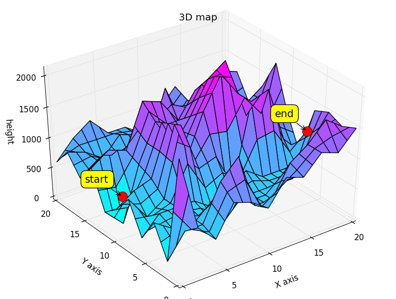
作图源码：

from mpl_toolkits.mplot3d import proj3d
from mpl_toolkits.mplot3d import Axes3D
import numpy as npheight3d = np.array([[2000,1400,800,650,500,750,1000,950,900,800,700,900,1100,1050,1000,1150,1300,1250,1200,1350,1500],                   [1100,900,700,625,550,825,1100,1150,1200,925,650,750,850,950,1050,1175,1300,1350,1400,1425,1450],                    [200,400,600,600,600,900,1200,1350,1500,1050,600,600,600,850,1100,1200,1300,1450,1600,1500,1400],                   [450,500,550,575,600,725,850,875,900,750,600,600,600,725,850,900,950,1150,1350,1400,1450],                   [700,600,500,550,600,550,500,400,300,450,600,600,600,600,600,600,600,850,1100,1300,1500],                    [500,525,550,575,600,575,550,450,350,475,600,650,700,650,600,600,600,725,850,1150,1450],                    [300,450,600,600,600,600,600,500,400,500,600,700,800,700,600,600,600,600,600,1000,1400],                    [550,525,500,550,600,875,1150,900,650,725,800,700,600,875,1150,1175,1200,975,750,875,1000],                    [800,600,400,500,600,1150,1700,1300,900,950,1000,700,400,1050,1700,1750,1800,1350,900,750,600],                   [650,600,550,625,700,1175,1650,1275,900,1100,1300,1275,1250,1475,1700,1525,1350,1200,1050,950,850],                   [500,600,700,750,800,1200,1600,1250,900,1250,1600,1850,2100,1900,1700,1300,900,1050,1200,1150,1100],                   [400,375,350,600,850,1200,1550,1250,950,1225,1500,1750,2000,1950,1900,1475,1050,975,900,1175,1450],                    [300,150,0,450,900,1200,1500,1250,1000,1200,1400,1650,1900,2000,2100,1650,1200,900,600,1200,1800],                    [600,575,550,750,950,1275,1600,1450,1300,1300,1300,1525,1750,1625,1500,1450,1400,1125,850,1200,1550],                    [900,1000,1100,1050,1000,1350,1700,1650,1600,1400,1200,1400,1600,1250,900,1250,1600,1350,1100,1200,1300],                   [750,850,950,900,850,1000,1150,1175,1200,1300,1400,1325,1250,1125,1000,1150,1300,1075,850,975,1100],                    [600,700,800,750,700,650,600,700,800,1200,1600,1250,900,1000,1100,1050,1000,800,600,750,900],                    [750,775,800,725,650,700,750,775,800,1000,1200,1025,850,975,1100,950,800,900,1000,1050,1100],                    [900,850,800,700,600,750,900,850,800,800,800,800,800,950,1100,850,600,1000,1400,1350,1300],                    [750,800,850,850,850,850,850,825,800,750,700,775,850,1000,1150,875,600,925,1250,1100,950],                   [600,750,900,1000,1100,950,800,800,800,700,600,750,900,1050,1200,900,600,850,1100,850,600]])fig = figure()
ax = Axes3D(fig)
X = np.arange(21)
Y = np.arange(21)
X, Y = np.meshgrid(X, Y)
Z = -20*np.exp(-0.2*np.sqrt(np.sqrt(((X-10)**2+(Y-10)**2)/2)))+20+np.e-np.exp((np.cos(2*np.pi*X)+np.sin(2*np.pi*Y))/2)
ax.plot_surface(X, Y, Z, rstride=1, cstride=1, cmap='cool')
ax.set_xlabel('X axis')
ax.set_ylabel('Y axis')
ax.set_zlabel('Z')
ax.set_title('3D map')point0 = [0,9,Z[0][9]] 
point1 = [20,7,Z[20][7]]ax.plot([point0[0]],[point0[1]],[point0[2]],'r',marker = u'o',markersize = 15)
ax.plot([point1[0]],[point1[1]],[point1[2]],'r',marker = u'o',markersize = 15)x0,y0,_ = proj3d.proj_transform(point0[0],point0[1],point0[2], ax.get_proj())
x1,y1,_ = proj3d.proj_transform(point1[0],point1[1],point1[2], ax.get_proj())label = pylab.annotate("start", xy = (x0, y0), xytext = (-20, 20),textcoords = 'offset points', ha = 'right', va = 'bottom',bbox = dict(boxstyle = 'round,pad=0.5', fc = 'yellow', alpha = 1),arrowprops = dict(arrowstyle = '->', connectionstyle = 'arc3,rad=0'),fontsize=15)
label2 = pylab.annotate("end", xy = (x1, y1), xytext = (-20, 20),textcoords = 'offset points', ha = 'right', va = 'bottom',bbox = dict(boxstyle = 'round,pad=0.5', fc = 'yellow', alpha = 1),arrowprops = dict(arrowstyle = '->', connectionstyle = 'arc3,rad=0'),fontsize=15)
def update_position(e):x2, y2, _ = proj3d.proj_transform(point0[0],point0[1],point0[2],ax.get_proj())label.xy = x2,y2label.update_positions(fig.canvas.renderer)x1,y1,_ =  proj3d.proj_transform(point1[0],point1[1],point1[2],ax.get_proj())label2.xy = x1,y1label2.update_positions(fig.canvas.renderer)fig.canvas.draw()fig.canvas.mpl_connect('button_release_event', update_position)

基本原理

蚂蚁 $k$ 根据各个城市间链接路径上的信息素浓度决定其下一个访问城市，设 $P_{ij}^k(t)$ 表示 $t$ 时刻蚂蚁 $k$ 从城市 $i$ 转移到矩阵 $j$ 的概率，其计算公式为

$P k i j = ⎧ ⎩ ⎨ [ τ i j ( t ) ] α \cdot [ η i j ( t ) ] β \sum s \in a l l o w k [ τ i s ( t ) ] α \cdot [ η i s ( t ) ] β 0 s \in a l l o w k s \notin a l l o w k$ $\begin{eqnarray*} P_{ij}^k=\begin{cases}\frac{[\tau_{ij}(t)]^{\alpha}\cdot[\eta_{ij}(t)]^{\beta}}{\sum_{s\in allow_k}[\tau_{is}(t)]^{\alpha}\cdot[\eta_{is}(t)]^{\beta}}\!&s\in allow_k \\0\!& s\notin allow_k\end{cases} \end{eqnarray*}$

计算完城市间的转移概率后，采用与遗传算法中一样的轮盘赌方法选择下一个待访问的城市。
当所有的蚂蚁完成一次循环后，各个城市间链接路径上的信息素浓度需进行更新，计算公式为

${τ i j (t + 1) = (1 - ρ) τ i j (t) + Δ τ i j Δ τ i j = \sum n k = 1 δ τ k i j$ $\begin{eqnarray*}\begin{cases}\tau_{ij}(t+1)=(1-\rho)\tau_{ij}(t)+\Delta\tau_{ij} \\\Delta\tau_{ij} = \sum_{k=1}^{n}\delta\tau_{ij}^k\end{cases} \end{eqnarray*}$

其中， $\Delta\tau_{ij}^k$ 表示第 $k$ 只蚂蚁在城市 $i$ 与城市 $j$ 连接路径上释放的信息素浓度； $\Delta\tau_{ij}$ 表示所有蚂蚁在城市 $i$ 与城市 $j$ 连接路径上释放的信息素浓度之和。
蚂蚁释放信息素的模型
$Δ τ k i j = {Q / L k, 0, 第 k 只蚂蚁从城市 i 访问城市 j 其他$ $\begin{eqnarray*} \Delta\tau_{ij}^k=\begin{cases}Q/L_k,&\mathrm{第k只蚂蚁从城市i访问城市j} \\0,&\mathrm{其他}\end{cases} \end{eqnarray*}$

程序代码：

import numpy as np
import matplotlib.pyplot as plt
%pylab
coordinates = np.array([[565.0,575.0],[25.0,185.0],[345.0,750.0],[945.0,685.0],[845.0,655.0],[880.0,660.0],[25.0,230.0],[525.0,1000.0],[580.0,1175.0],[650.0,1130.0],[1605.0,620.0],[1220.0,580.0],[1465.0,200.0],[1530.0,  5.0],[845.0,680.0],[725.0,370.0],[145.0,665.0],[415.0,635.0],[510.0,875.0],[560.0,365.0],[300.0,465.0],[520.0,585.0],[480.0,415.0],[835.0,625.0],[975.0,580.0],[1215.0,245.0],[1320.0,315.0],[1250.0,400.0],[660.0,180.0],[410.0,250.0],[420.0,555.0],[575.0,665.0],[1150.0,1160.0],[700.0,580.0],[685.0,595.0],[685.0,610.0],[770.0,610.0],[795.0,645.0],[720.0,635.0],[760.0,650.0],[475.0,960.0],[95.0,260.0],[875.0,920.0],[700.0,500.0],[555.0,815.0],[830.0,485.0],[1170.0, 65.0],[830.0,610.0],[605.0,625.0],[595.0,360.0],[1340.0,725.0],[1740.0,245.0]])def getdistmat(coordinates):num = coordinates.shape[0]distmat = np.zeros((52,52))for i in range(num):for j in range(i,num):distmat[i][j] = distmat[j][i]=np.linalg.norm(coordinates[i]-coordinates[j])return distmatdistmat = getdistmat(coordinates)numant = 40 #蚂蚁个数
numcity = coordinates.shape[0] #城市个数
alpha = 1   #信息素重要程度因子
beta = 5    #启发函数重要程度因子
rho = 0.1   #信息素的挥发速度
Q = 1iter = 0
itermax = 250etatable = 1.0/(distmat+np.diag([1e10]*numcity)) #启发函数矩阵，表示蚂蚁从城市i转移到矩阵j的期望程度
pheromonetable  = np.ones((numcity,numcity)) # 信息素矩阵
pathtable = np.zeros((numant,numcity)).astype(int) #路径记录表distmat = getdistmat(coordinates) #城市的距离矩阵lengthaver = np.zeros(itermax) #各代路径的平均长度
lengthbest = np.zeros(itermax) #各代及其之前遇到的最佳路径长度
pathbest = np.zeros((itermax,numcity)) # 各代及其之前遇到的最佳路径长度while iter < itermax:# 随机产生各个蚂蚁的起点城市if numant <= numcity:#城市数比蚂蚁数多pathtable[:,0] = np.random.permutation(range(0,numcity))[:numant]else: #蚂蚁数比城市数多，需要补足pathtable[:numcity,0] = np.random.permutation(range(0,numcity))[:]pathtable[numcity:,0] = np.random.permutation(range(0,numcity))[:numant-numcity]length = np.zeros(numant) #计算各个蚂蚁的路径距离for i in range(numant):visiting = pathtable[i,0] # 当前所在的城市#visited = set() #已访问过的城市，防止重复#visited.add(visiting) #增加元素unvisited = set(range(numcity))#未访问的城市unvisited.remove(visiting) #删除元素for j in range(1,numcity):#循环numcity-1次，访问剩余的numcity-1个城市#每次用轮盘法选择下一个要访问的城市listunvisited = list(unvisited)probtrans = np.zeros(len(listunvisited))for k in range(len(listunvisited)):probtrans[k] = np.power(pheromonetable[visiting][listunvisited[k]],alpha)\*np.power(etatable[visiting][listunvisited[k]],alpha)cumsumprobtrans = (probtrans/sum(probtrans)).cumsum()cumsumprobtrans -= np.random.rand()k = listunvisited[find(cumsumprobtrans>0)[0]] #下一个要访问的城市pathtable[i,j] = kunvisited.remove(k)#visited.add(k)length[i] += distmat[visiting][k]visiting = klength[i] += distmat[visiting][pathtable[i,0]] #蚂蚁的路径距离包括最后一个城市和第一个城市的距离#print length# 包含所有蚂蚁的一个迭代结束后，统计本次迭代的若干统计参数lengthaver[iter] = length.mean()if iter == 0:lengthbest[iter] = length.min()pathbest[iter] = pathtable[length.argmin()].copy()      else:if length.min() > lengthbest[iter-1]:lengthbest[iter] = lengthbest[iter-1]pathbest[iter] = pathbest[iter-1].copy()else:lengthbest[iter] = length.min()pathbest[iter] = pathtable[length.argmin()].copy()    # 更新信息素changepheromonetable = np.zeros((numcity,numcity))for i in range(numant):for j in range(numcity-1):changepheromonetable[pathtable[i,j]][pathtable[i,j+1]] += Q/distmat[pathtable[i,j]][pathtable[i,j+1]]changepheromonetable[pathtable[i,j+1]][pathtable[i,0]] += Q/distmat[pathtable[i,j+1]][pathtable[i,0]]pheromonetable = (1-rho)*pheromonetable + changepheromonetableiter += 1 #迭代次数指示器+1#观察程序执行进度，该功能是非必须的if (iter-1)%20==0: print iter-1# 做出平均路径长度和最优路径长度        
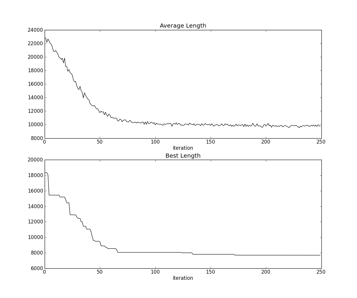
fig,axes = plt.subplots(nrows=2,ncols=1,figsize=(12,10))
axes[0].plot(lengthaver,'k',marker = u'')
axes[0].set_title('Average Length')
axes[0].set_xlabel(u'iteration')axes[1].plot(lengthbest,'k',marker = u'')
axes[1].set_title('Best Length')
axes[1].set_xlabel(u'iteration')
fig.savefig('Average_Best.png',dpi=500,bbox_inches='tight')
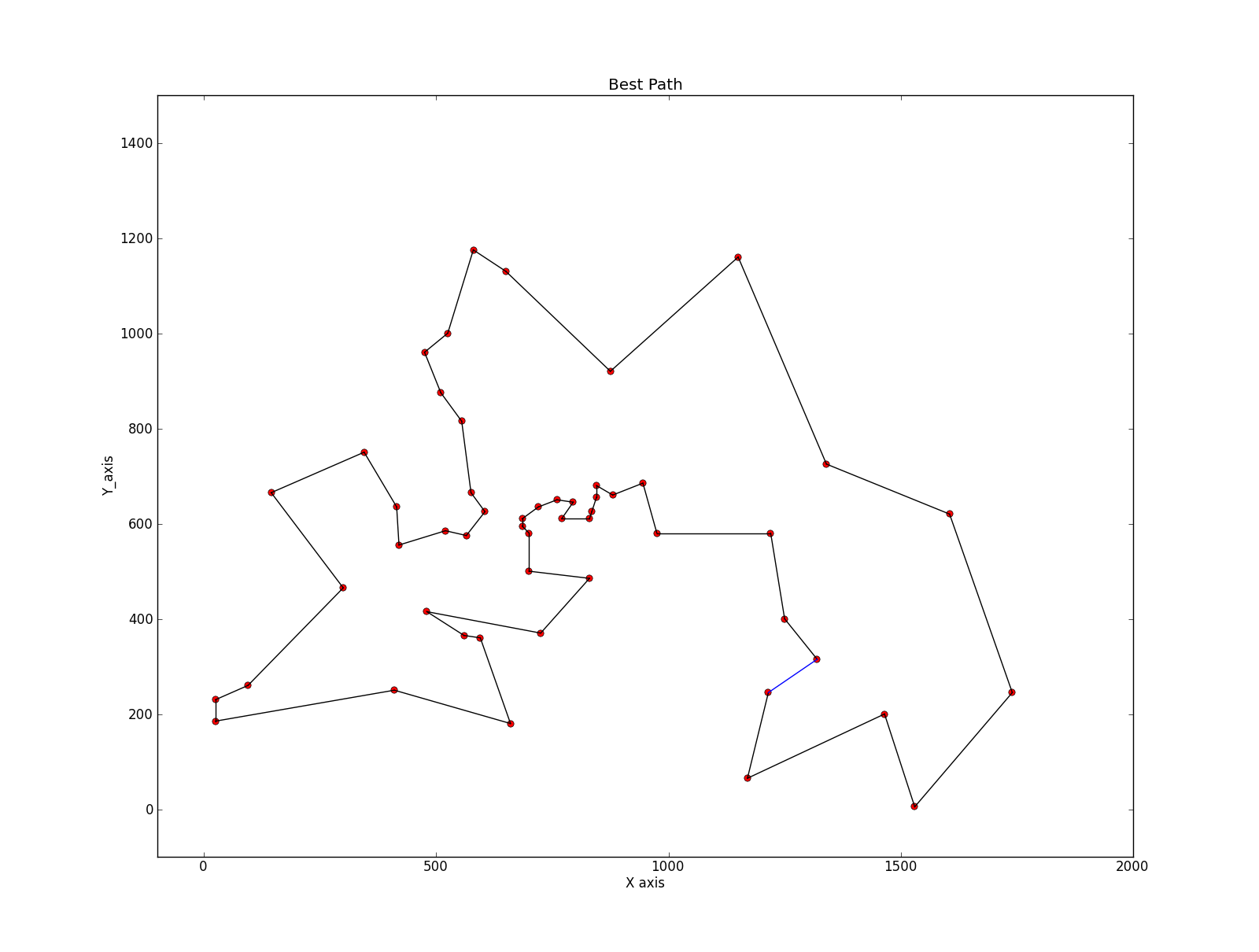
plt.close()#作出找到的最优路径图
bestpath = pathbest[-1]plt.plot(coordinates[:,0],coordinates[:,1],'r.',marker=u'$\cdot$')
plt.xlim([-100,2000])
plt.ylim([-100,1500])for i in range(numcity-1):#m,n = bestpath[i],bestpath[i+1]print m,nplt.plot([coordinates[m][0],coordinates[n][0]],[coordinates[m][1],coordinates[n][1]],'k')
plt.plot([coordinates[bestpath[0]][0],coordinates[n][0]],[coordinates[bestpath[0]][1],coordinates[n][1]],'b')ax=plt.gca()
ax.set_title("Best Path")
ax.set_xlabel('X axis')
ax.set_ylabel('Y_axis')plt.savefig('Best Path.png',dpi=500,bbox_inches='tight')
plt.close()