基于图神经网络的节点表征学习

节点表征

在图的节点预测或者边预测任务中, 需要先构造节点表征, 这一点尤为重要
- 节点的属性可以是类别型, 也可以是数值型
以下分别使用MLP, GCN, GAT, GraphSage来进行节点预测
- 1.获取并分析数据集、构建一个方法用于分析节点表征的分布
- 2.使用MLP进行节点预测
- 3.分别使用GCN, GAT, GraphSage进行节点预测
- 4.比较4个模型在节点预测的差异

1. 获取并分析数据集

数据转换在将数据输入神经网络之前修改数据, 可以实现数据的规范化和数据增强
- NormalizeFeatures: 进行节点特征归一化, 使各节点特征的和为1
- 其他转换方法

from torch_geometric.datasets import Planetoid
from torch_geometric.transforms import NormalizeFeaturesdataset = Planetoid(root='./input/Cora', name='Cora', transform=NormalizeFeatures())print(f'dataset: {dataset}')
print(f'number of graphs: {len(dataset)}')
print(f'number of features: {dataset.num_node_features}')
print(f'number of classes: {dataset.num_classes}')data = dataset[0]
print(f'data: {data}')
print(f'{"="*10}some statistics about the graph{"="*10}')
print(f'number of nodes: {data.num_nodes}')
print(f'number of edges: {data.num_edges}')
print(f'average node degree: {data.num_edges / data.num_nodes:.2f}')
print(f'training node label rate: {int(data.train_mask.sum()) / data.num_nodes:.2f}')
print(f'contains isolated nodes: {data.contains_isolated_nodes()}')
print(f'contains self-loops: {data.contains_self_loops()}')
print(f'is undirected: {data.is_undirected()}')

数据分析结果

2. 可视化节点表征分布

利用TSNE将高维节点表征嵌入到二位平面空间

import matplotlib.pyplot as plt
from sklearn.manifold import TSNEdef visualize(out, color):z = TSNE(n_components=2).fit_transform(out.detach().cpu().numpy())plt.figure(figsize=(10, 10))plt.xticks([])plt.yticks([])plt.scatter(z[:, 0], z[:, 1], s=70, c=color, cmap='Set2')plt.show()

3. MLP在图节点分类中的应用

import torch
from torch.nn import Linear
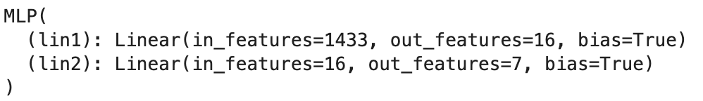
import torch.nn.functional as Fclass MLP(torch.nn.Module):"""MLP的参数由输入维度, 隐层维度, 输出维度构成"""def __init__(self, in_channels, hidden_channels, out_channels, seed=2021):super(MLP, self).__init__()torch.manual_seed(seed)self.lin1 = Linear(in_channels, hidden_channels)self.lin2 = Linear(hidden_channels, out_channels)def forward(self, x):x = self.lin1(x)x = x.relu()x = F.dropout(x, p=0.5, training=self.training)x = self.lin2(x)return xmodel = MLP(dataset.num_features, 16, dataset.num_classes)
print(model)

MLP模型

定义训练和测试函数

criterion = torch.nn.CrossEntropyLoss()
optimizer = torch.optim.Adam(model.parameters(), lr=0.01, weight_decay=5e-4)def train():model.train()optimizer.zero_grad()out = model(data.x)_, pred = out.max(dim=1)correct = float(pred[data.train_mask].eq(data.y[data.train_mask]).sum().item())acc = correct / data.train_mask.sum().item()loss = criterion(out[data.train_mask], data.y[data.train_mask])loss.backward()optimizer.step()return loss, accdef test():model.eval()_, pred = model(data.x).max(dim=1)correct = float(pred[data.test_mask].eq(data.y[data.test_mask]).sum().item())acc = correct / data.test_mask.sum().item()return acc

训练, 测试

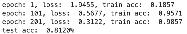
# 训练
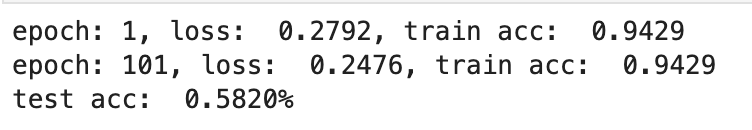
for epoch in range(200):loss, acc = train()if epoch % 100 == 0:print(f'epoch: {epoch + 1}, loss: {loss: .4f}, train acc: {acc: .4f}')#  测试
acc = test()
print(f'test acc: {acc: .4f}%')

MLP结果

4.卷积图神经网络GCN

构造, 将MLP的Linear换成GCNConv

from torch_geometric.nn import GCNConvclass GCN(torch.nn.Module):def __init__(self, in_channels, hidden_channels, out_channels, seed=2021):super(GCN, self).__init__()torch.manual_seed(seed)self.conv1 = GCNConv(in_channels, hidden_channels)self.conv2 = GCNConv(hidden_channels, out_channels)def forward(self, x, edge_index):x = self.conv1(x, edge_index)x = x.relu()x = F.dropout(x, p=0.5, training=self.training)x = self.conv2(x, edge_index)return x

通过TSNE对图进行降维可视化

model = GCN(in_channels=dataset.num_features, hidden_channels=16, out_channels=dataset.num_classes)out = model(data.x, data.edge_index)
visualize(out, color=data.y)

图可视化

GCN训练, 测试

optimizer = torch.optim.Adam(model.parameters(), lr=0.01, weight_decay=5e-4)
criterion = torch.nn.CrossEntropyLoss()def train():model.train()optimizer.zero_grad()out = model(data.x, data.edge_index)_, pred = out.max(dim=1)correct = float(pred[data.train_mask].eq(data.y[data.train_mask]).sum().item())acc = correct / data.train_mask.sum().item()loss = criterion(out[data.train_mask], data.y[data.train_mask])loss.backward()optimizer.step()return loss, accdef test():model.eval()_, pred = model(data.x, data.edge_index).max(dim=1)correct = float(pred[data.test_mask].eq(data.y[data.test_mask]).sum().item())acc = correct / data.test_mask.sum().item()return acc# 训练
for epoch in range(300):loss, acc = train()if epoch % 100 == 0:print(f'epoch: {epoch + 1}, loss: {loss: .4f}, train acc: {acc: .4f}')#  测试
acc = test()
print(f'test acc: {acc: .4f}%')

GCN结果

使用GCN分类之后进行可视化

model.eval()
out = model(data.x, data.edge_index)
visualize(out, color=data.y)

分类之后可视化

5、图注意力神经网络

5.1 GAT的定义

公式:
$x_i' = \alpha_{i,i}\Theta X_i - \sum\limits_{j \in N_{(i)}} \alpha_{i,j}\Theta_j,$
注意力系数为 $\alpha_{i,j}$
$\alpha_{i,j} = \frac{exp(LeakyReLU(a^T[\Theta X_i || \Theta X_j]))}{\sum_{k \in N_{(i)} U {i}} exp(LeakyReLU(a^T[\Theta X_i || \Theta X_k]))}$
PyG的GATConv构造函数接口

GATConv(in_channels: Union[int, Tuple[int, int]], out_channels: int, heads: int = 1, concat: bool = True, negative_slope: float = 0.2, dropout: float = 0.0, add_self_loops: bool = True, bias: bool = True, **kwargs
)

GAT图神经网络的构造

import torch
from torch.nn import Linear
import torch.nn.functional as F
from torch_geometric.nn import GATConvclass GAT(torch.nn.Module):def __init__(self, in_channels, hidden_channels, out_channels, seed=2021):super(GAT, self).__init__()torch.manual_seed(seed)self.conv1 = GATConv(in_channels, hidden_channels)self.conv2 = GATConv(hidden_channels, out_channels)def forward(self, x, edge_index):x = self.conv1(x, edge_index)x = x.relu()x = F.dropout(x, p=0.5, training=self.training)x = self.conv2(x, edge_index)return x

GAT输出的图可视化

model = GAT(in_channels=dataset.num_features, hidden_channels=16, out_channels=dataset.num_classes)out = model(data.x, data.edge_index)
visualize(out, color=data.y)

GAT输出可视化

GAT 训练, 测试

optimizer = torch.optim.Adam(model.parameters(), lr=0.01, weight_decay=5e-4)
criterion = torch.nn.CrossEntropyLoss()def train():model.train()optimizer.zero_grad()out = model(data.x, data.edge_index)_, pred = out.max(dim=1)correct = float(pred[data.train_mask].eq(data.y[data.train_mask]).sum().item())acc = correct / data.train_mask.sum().item()loss = criterion(out[data.train_mask], data.y[data.train_mask])loss.backward()optimizer.step()return loss, accdef test():model.eval()_, pred = model(data.x, data.edge_index).max(dim=1)correct = float(pred[data.test_mask].eq(data.y[data.test_mask]).sum().item())acc = correct / data.test_mask.sum().item()return acc# 训练
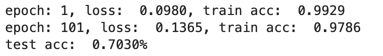
for epoch in range(200):loss, acc = train()if epoch % 100 == 0:print(f'epoch: {epoch + 1}, loss: {loss: .4f}, train acc: {acc: .4f}')#  测试
acc = test()
print(f'test acc: {acc: .4f}%')

GAT测试结果

GAT分类可视化

model.eval()
out = model(data.x, data.edge_index)
visualize(out, color=data.y)`

GAT分类可视化

6. 总结

MLP: acc 58.2%
GCN: acc 81.2%
GAT: acc 70.3%
由以上结果可以看出, MLP的模型过于简单, 他只考虑了节点自身属性, 忽略了节点的连接关系, 所以拟合效果很差
GCN和GAT考虑了节点自身和周围邻居节点的属性, 结果优于MLP

6.1 GCN 与 GAT 相同点

都基于图神经网络的节点表征的学习遵循消息传递范式
GCN与GAT都对邻居节点做归一化和线性变换
在邻居节点信息聚合阶段都将变换后的邻居节点信息做求和聚合；
在中心节点信息变换阶段只是简单返回邻居节点信息聚合阶段的聚合结
果

6.2 GCN 与 GAT 不同点

GCN与GAT的区别在于邻居节点信息聚合过程中的归一化方法不同
- GCN根据中心节点与邻居节点的度计算归一化系数，GAT根据中心节点与邻居节点的相似度计算归一化系数。
- GCN的归一化方式依赖于图的拓扑结构，不同节点其自身的度不同、其邻居的度也不同，在一些应用中可能会影响泛化能力。
- GAT者的归一化方式依赖于中心节点与邻居节点的相似度，相似度是训练得到的，因此不受图的拓扑结构的影响，在不同的任务中都会有较好的泛化表现。

7. GraphSage

7.1 采样(sampling.py)

对邻居的采样
对邻居的聚合操作
sampling: 一阶采样
multihop_sampling: 利用sampling进行多

import numpy as np
def sampling(src_nodes, sample_num, neighbor_table):"""根据源节点采样指定数量的邻居节点, 使用有放回采样; Arguments:src_nodes {list, ndarray} -- 源节点列表sample_num {int} -- 需要采样的节点数neighbor_table {dict} -- 节点到其邻居节点的映射表Returns:np.ndarray -- 采样结果构成的列表"""results = []for sid in src_nodes:# 有放回采样res = np.random.choice(neighbor_table[sid], size=(sample_num, ))results.append(res)return np.asarray(results).flatten()def multihop_sampling(src_nodes, sample_nums, neighbor_table):"""根据源节点进行多阶采样Arguments:src_nodes {list, ndarray} -- 源节点列表sample_num {int} -- 需要采样的节点数neighbor_table {dict} -- 节点到其邻居节点的映射表Returns:[list of ndarray] -- 每一阶采样的结果"""sampling_result = [src_nodes]for k, hopk_num in enumerate(sample_nums):hopk_result = sampling(sample_result[k], hopk_num, neighbor_table)sampling_result.append(hopk_result)return sampling_result

7.2 聚合(net.py)

使用神经网络实现
neighbor_feature表示需要聚合的邻居节点的特征, 它的维度为 $N_{src} * N_{neighbor} * D_{in}$
- $N_{src}$ : 源节点的数量
- $N_neighbor$ : 表示邻居节点的数量
- $D_in$ : 表示输入特征的维度
将邻居节点的特征通过线性变换得到隐藏层特征, 进而求和, 均值, 最大值等聚合操作, 得到 $N_{src} * D_{in}$ 维的输出

import torch
import torch.nn as nn
import torch.nn.functional as F
import torch.nn.init as initclass NeighborAggregator(nn.Module):def __init__(self, input_dim, output_dim, use_bias=False, aggr_method="mean"):super(NeighborAggregator, self).__init__()self.input_dim = input_dimself.output_dim = output_dimself.use_bias = use_biasself.aggr_method = aggr_methodself.weight = nn.Parameter(torch.Tensor(input_dim, output_dim))if self.use_bias:self.bias = nn.Parameter(torch.Tensor(self.output_dim))self.reset_parameters()def reset_parameters(self):init.kaiming_uniform_(self.weight)if self.use_bias:init.zeros_(self.bias)def forward(self, neighbor_feature):if self.aggr_method == "mean":aggr_neighbor = neighbor_feature.mean(dim=1)elif self.aggr_method == "sum":aggr_neighbor = neighbor_feature.sum(dim=1)elif self.aggr_method == "max":aggr_neighbor = neighbor_feature.max(dim=1)else:raise ValueError(f"Unknown aggr type, expected sum, max, or mean, but got {self.aggr_method}")neighbor_hidden = torch.matmul(aggr_neighbor, self.weight)if self.use_bias:neighbor_hidden += self.biasreturn neighbor_hiddendef extra_repr(self):return f'in_features={self.input_dim}, out_features={self.output_dim}, aggr_method={self.aggr_method}'

3. GraphSage模型构建(net.py)

Concatenate neighbor embedding and neighbor embedding
定义SageGCN
- neighbor_hidden: 由self.aggregator计算得到, 计算的是公式: $W_k \cdot AGG(\{h_u^{k-1}, \forall_u \in N_{(v)}\})$ , 包括 mean, sum, pool
- self_hidden: 计算的是公式: $B_kh_v^{k-1}$ , 侧重于节点自身的属性, 包括sum(矩阵相加), concat(矩阵拼接)

class SageGCN(nn.Module):def __init__(self, input_dim, hidden_dim, activation=F.relu, aggr_neighbor_method='mean', aggr_hidden_method='sum'):"""Args:input_dim: 输入特征的维度hidden_dim: 隐层特征的维度，当aggr_hidden_method=sum, 输出维度为hidden_dim当aggr_hidden_method=concat, 输出维度为hidden_dim*2activation: 激活函数aggr_neighbor_method: 邻居特征聚合方法，["mean", "sum", "max"]aggr_hidden_method: 节点特征的更新方法，["sum", "concat"]"""super(SageGCN, self).__init__()assert aggr_neighbor_method in ['mean', 'sum', 'max']assert aggr_hidden_method in ['sum', 'concat']self.input_dim = input_dimself.hidden_dim = hidden_dimself.aggr_neighbor_method = aggr_neighbor_methodself.aggr_hidden_method = aggr_hidden_methodself.activation = activationself.aggregator = NeighborAggregator(input_dim, hidden_dim, aggr_method=aggr_neighbor_method)self.b = nn.Parameter(torch.Tensor(input_dim, hidden_dim))self.reset_parameters()def reset_parameters(self):init.kaiming_uniform_(self.b)def forward(self, src_node_features, neighbor_node_features):neighbor_hidden = self.aggregator(neighbor_node_features)self_hidden = torch.matmul(src_node_features, self.b)if self.aggr_hidden_method == 'sum':hidden = self_hidden + neighbor_hiddenelif self.aggr_hidden_method == 'concat':hidden = torch.cat([self_hidden, neighbor_hidden], dim=1)else:raise ValueError(f"Expected sum or concat, got {self.aggr_hidden}")if self.activation:return self.activation(hidden)else:return hiddendef extra_repr(self):output_dim = self.hidden_dim if self.aggr_hidden_method == "sum" else self.hidden_dim * 2return f'in_features={self.input_dim}, out_features={output_dim}, aggr_hidden_method={self.aggr_hidden_method}'

定义GraphSage

class GraphSage(nn.Module):def __init__(self, input_dim, hidden_dim, num_neighbors_list):super(GraphSage, self).__init__()self.input_dim = input_dimself.hidden_dim = hidden_dimself.num_neighbors_list = num_neighbors_listself.num_layers = len(num_neighbors_list)self.gcn = nn.ModuleList()self.gcn.append(SageGCN(input_dim, hidden_dim[0]))for index in range(0, len(hidden_dim) - 2):self.gcn.append(SageGCN(hidden_dim[index], hidden_dim[index + 1]))self.gcn.append(SageGCN(hidden_dim[-2], hidden_dim[-1], activation=None))def forward(self, node_feature_list):hidden = node_feature_listfor l in range(self.num_layers):next_hidden = []gcn = self.gcn[l]for hop in range(self.num_layers - l):src_node_features = hidden[hop]src_node_num = len(src_node_features)neighbor_node_features = hidden[hop + 1].view((src_node_num, self.num_neighbors_list[hop], -1))h = gcn(src_node_features, neighbor_node_features)next_hidden.append(h)hidden = next_hiddenreturn hidden[0]def extra_repr(self):return f'in_features={self.input_dim}, num_neighbors_list={self.num_neighbors_list}'

构建模型

INPUT_DIM = dataset.num_features    # 输入维度
# Note: 采样的邻居阶数需要与GCN的层数保持一致
HIDDEN_DIM = [128, 7]   # 隐藏单元节点数
NUM_NEIGHBORS_LIST = [10, 10]   # 每阶采样邻居的节点数
assert len(HIDDEN_DIM) == len(NUM_NEIGHBORS_LIST)model = GraphSage(input_dim=INPUT_DIM, hidden_dim=HIDDEN_DIM, num_neighbors_list=NUM_NEIGHBORS_LIST)
print(model)