在机器学习中,模型更容易从具有正态分布特性的数据中学习到有用特征。但我们经常会发现有些特征存在长尾分布,对于这种偏态分布数据,需要进行特殊的处理,本文首先观察特征分布情况,然后以量化的方式评估数据偏态程度从而挑选出偏态数据,最后对偏态数据进行对数化处理,对比处理前后的特征分布。
通过箱线图观察不同特征的分布情况
# 查看特征的数据倾斜情况
# 丢弃y值
all_features = df_train.drop(['label'], axis=1)# 找出所有的数值型变量
numeric_dtypes = ['int16', 'int32', 'int64', 'float16', 'float32', 'float64']
numeric = []
for i in df_data.columns:if df_data[i].dtype in numeric_dtypes:numeric.append(i)# 对所有的数值型变量绘制箱体图
sns.set_style("white")
f, ax = plt.subplots(figsize=(20, 100))
ax.set_xscale("log")
ax = sns.boxplot(data=df_data[numeric] , orient="h", palette="Set1")
ax.xaxis.grid(False)
ax.set(ylabel="Feature names")
ax.set(xlabel="Numeric values")
ax.set(title="Numeric Distribution of Features")
sns.despine(trim=True, left=True)

通过量化指标-偏态系数找出倾斜较大的特征列
# 找出明显偏态的数值型变量
skew_features = df_train[numeric].apply(lambda x: x.skew()).sort_values(ascending=False)high_skew = skew_features[skew_features > 0.5]
skew_index = high_skew.indexprint("本数据集中有 {} 个数值型变量的 Skew > 0.5 :".format(high_skew.shape[0]))
skewness = pd.DataFrame({'Skew' :high_skew})
skew_features.head(10)

观察不同标签下特征的分布情况,以及经过对数化处理的特征分布情况
fig, (ax1, ax2) = plt.subplots(2,1, figsize=(20,10))sns.histplot(data=df_train+1, x="max_call_cnt/called_cnt", hue="label",bins=20, ax=ax1)
ax1.set_title("Origin feature distribution")
sns.histplot(data=df_train+1, x="max_call_cnt/called_cnt", hue="label",bins=20,log_scale=10, ax=ax2)
ax2.set_title("log feature distribution")plt.show()