数据挖掘之聚类分析（Cluster Analysis）

1.Motivations（目的）

Identify grouping structure of data so that objects within the same group are closer (more similar) to each other while farther (less similar) to those in different groups
- Various distance/proximity functions
- intra-cluster distance vs. inter-cluster distance
Unsupervised learning: used for data exploration
- Can also be adapted for supervised learning purpose
Types of cluster analysis
- Partitional vs. Hierarchical: one point can belong to one or multiple clusters
- kmeans algorithm vs. HAC (Hierarchical Agglomerative Clustering) algorithm

中：

识别数据的分组结构，以便同一组内的对象彼此更接近（更相似），而与不同组中的对象更远（更不相似）
- 各种距离/接近功能
- 簇内距离与簇间距离
无监督学习：用于数据探索
- 也可以适应监督学习目的
聚类分析的类型
- 分区与分层：一个点可以属于一个或多个集群
- kmeans算法与HAC（Hierarchical Agglomerative Clustering）算法

2.Partitional vs. Hierarchical Clustering（分区与分层聚类）

$[外链图片转存失败(img-jTROiuj3-1562291299486)(C:\Users\lenovo\AppData\Roaming\Typora\typora-user-images\1562220427447.png)]$

3.Major Applications of Cluster Analysis

Data sampling: use centroid as the representative samples
- Centroid: center of mass which is caculated as the (arithmetic) mean of all the data points in the same cluster (separately for each dimension)
Marketing segmentation analysis: help marketers segment their customer bases and develop targeted marketing programs
Insurance: identify groups of motor insurance policy holders with a higher average claim cost
Microarray analysis for biomedical research: A high throughput technology which allows testing thousand of genes simultaneously in different disease states

中:

聚类分析的主要应用

数据采样：使用质心作为代表性样本
- 质心：质心，计算为同一簇中所有数据点的（算术）平均值（每个维度分别）
营销细分分析：帮助营销人员细分客户群并制定有针对性的营销计划
保险：确定具有较高平均索赔成本的汽车保险保单持有人群体
用于生物医学研究的微阵列分析：一种高通量技术，允许在不同疾病状态下同时测试数千个基因

4.Distance Functions

Minkowski
Manhattan
Euclidean distance

$[外链图片转存失败(img-nibEjViE-1562291299488)(C:\Users\lenovo\AppData\Roaming\Typora\typora-user-images\1562222191249.png)]$

5. Cluster Validity Evaluation

SSE (Sum of Square Error): most common measure

$[外链图片转存失败(img-I6jLCv5v-1562291299489)(C:\Users\lenovo\AppData\Roaming\Typora\typora-user-images\1562222168396.png)]$

Cluster cohesion
SSE is a monotonically decreasing function of number of clusters. Therefore it can be used to compare cluster performance only for similar number of clusters

中：

SSE（平方误差之和）：最常见的度量
集群凝聚力
SSE是群集数量的单调递减函数。因此，它可用于仅针对相似数量的群集比较群集性能

6.Objective Function for Kmeans Clustering: SSE（Kmeans聚类的目标函数：SSE）

Also known as loss/cost function
Goal of Kmeans method is to
- Minimize SSE of within-cluster variance
- Same as the sum of Euclidean distance between all data points with their respective cluster centroids
Therefore no needs to set the distance function for Kmeans method

中：

也称为损失/成本函数
Kmeans方法的目标是
- 最小化群内方差的SSE
- 与所有数据点之间的欧几里德距离与其各自的聚类质心的总和相同
因此无需为Kmeans方法设置距离函数

7.Model Preprocessing（模型预处理）

Data standardization, normalization, rescale
- Applies to all algorithms based on distance: KNN
Remove or impute missing values
Detection and removal of noisy data and outliers
Transformation of categorical attributes into numerical attributes (opposite to association rule mining)

中：

数据标准化，规范化，重新缩放
- 适用于基于距离的所有算法：KNN
删除或估算缺失值
检测和消除噪声数据和异常值
将分类属性转换为数字属性（与关联规则挖掘相反）

8.Animation of How kmeans Algorithm works（kmeans算法如何工作的动画）

在这里插入图片描述

9.Summary of kmeans and HAC（kmeans和HAC摘要）

Kmeans
- Randomly assign k centroids
- Assign all data points to their closest centroids
- Update centroid assignments
- Repeat the previous two steps until centroids are stable
HAC
- Treat each data point as a cluster
- Compute the pairwise distance matrix for all clusters
- Merge closer clusters into a larger one and update the distance matrix
- keep repeating the previous step until there is only one cluster left
- Opposite: HDC (Hierarchical Divisive Clustering)

中：

K均值
- 随机分配k个质心
- 将所有数据点分配给最近的质心
- 更新质心分配
- 重复前两个步骤，直到质心稳定
HAC
- 将每个数据点视为一个集群
- 计算所有聚类的成对距离矩阵
- 将更近的聚类合并为更大的聚类并更新距离矩阵
- 继续重复上一步，直到只剩下一个簇
- 相反：HDC（分层分裂聚类）

10.Defintion of Inter-Cluster Distance（群间距离的定义）

Single linkage: minimal pairwise distance between data points belonging to different clusters
Complete linkage: maximal pairwise distance between data points belonging to different clusters
Average linkage method: average pairwise distance between all data points belonging to different clusters
Centroid linkage method: pairwise distance between centroids of different clusters

中：

单链接：属于不同群集的数据点之间的最小成对距离
完全链接：属于不同簇的数据点之间的最大成对距离
平均连锁方法：属于不同聚类的所有数据点之间的平均成对距离
质心联动方法：不同聚类的质心之间的成对距离

11.Model Parameters（模型参数）

Algorithm-specific
- kmeans
  - Number of clusters: Elbow method to estimate
  - Initial choice of cluster centers (centroid)
    - Kmeans method is guaranteed to converge but not guaranteed to converge to global optimial
  - Maximal number of repeats
- Hierarchical clustering
  - Distance function between data points
  - Definition of intercluster distance: single vs. complete vs. average vs. centroid linkage
  - Number of clusters to output (needed after clustering)
算法的具体
- k均值
  - 簇数：肘法估算
  - 群集中心的初始选择（质心）
    - Kmeans方法保证收敛但不保证收敛到全局优化
  - 最大重复次数
- 分层聚类
  - 数据点之间的距离函数
  - 集群间距离的定义：单对与完全对比平均与质心联系
  - 要输出的簇数（在群集后需要）

12.Comparison Between Kmeans and HAC (1)

Objective function
- Kmeans: sum of square difference between data points and their respective centroid (within SS)
- HAC: no objective function
Parameter setting
- Kmeans: need to specify number of clusters prior to running aglorithm
- HAC: no need to choose number of clusters a priori; can choose after fact
Performance
- Kmeans: Fast with linear time complexity O(N) (ñ: number of data points)
- HAC: Slow with quadratic complexity O(N^2)
- Hybrid approach: run Kmeans first to reduce dataset size and then HAC to cluster

中：

目标功能
- Kmeans：数据点与其各自质心之间的平方差的总和（在SS内）
- HAC：没有客观功能
参数设置
- Kmeans：需要在运行aglorithm之前指定簇数
- HAC：无需先验地选择集群数量; 事后可以选择
性能
- Kmeans：线性时间复杂度快 O （N）(ñ：数据点数）
- HAC：二次复杂性缓慢 O （N^2）
- 混合方法：首先运行Kmeans以减少数据集大小，然后运行HAC以进行群集

13.Comparison Between Kmeans and HAC (2)

Structure of clusters
- Kmeans: works best with sphere clusters with similar size
- HAC: works with clusters of different size and shape
  - Depending on inter-cluster distance definition
  - Single-linkage method: clusters of different size; prone to outliers
  - Complete-linkage method: clusters of similar size; prone to outliers
  - Average/Centroid linkage: resist outliers
- Both methods couldn’t deal well with clusters of different densities: DBScan
Both methods mostly work with numerical attributes only (contrary to association rule mining)

14.Demo(1)

14.1 Demo Dataset: USArrests

Crime dataset:
- Arrests per 100,000 residents for assault, murder, and rape in each of the 50 US states in 1973
- Percent of the population living in urban areas

> library(datasets)
> str(USArrests)
'data.frame':	50 obs. of  4 variables:$ Murder  : num  13.2 10 8.1 8.8 9 7.9 3.3 5.9 15.4 17.4 ...$ Assault : int  236 263 294 190 276 204 110 238 335 211 ...$ UrbanPop: int  58 48 80 50 91 78 77 72 80 60 ...$ Rape    : num  21.2 44.5 31 19.5 40.6 38.7 11.1 15.8 31.9 25.8 ...
> row.names(USArrests)[1] "Alabama"        "Alaska"         "Arizona"        "Arkansas"       "California"     "Colorado"      [7] "Connecticut"    "Delaware"       "Florida"        "Georgia"        "Hawaii"         "Idaho"         
[13] "Illinois"       "Indiana"        "Iowa"           "Kansas"         "Kentucky"       "Louisiana"     
[19] "Maine"          "Maryland"       "Massachusetts"  "Michigan"       "Minnesota"      "Mississippi"   
[25] "Missouri"       "Montana"        "Nebraska"       "Nevada"         "New Hampshire"  "New Jersey"    
[31] "New Mexico"     "New York"       "North Carolina" "North Dakota"   "Ohio"           "Oklahoma"      
[37] "Oregon"         "Pennsylvania"   "Rhode Island"   "South Carolina" "South Dakota"   "Tennessee"     
[43] "Texas"          "Utah"           "Vermont"        "Virginia"       "Washington"     "West Virginia" 
[49] "Wisconsin"      "Wyoming"

14.2 Data Preprocess

> sum(!complete.cases(USArrests))
[1] 0
> summary(USArrests)Murder          Assault         UrbanPop          Rape      Min.   : 0.800   Min.   : 45.0   Min.   :32.00   Min.   : 7.30  1st Qu.: 4.075   1st Qu.:109.0   1st Qu.:54.50   1st Qu.:15.07  Median : 7.250   Median :159.0   Median :66.00   Median :20.10  Mean   : 7.788   Mean   :170.8   Mean   :65.54   Mean   :21.23  3rd Qu.:11.250   3rd Qu.:249.0   3rd Qu.:77.75   3rd Qu.:26.18  Max.   :17.400   Max.   :337.0   Max.   :91.00   Max.   :46.00  
> df <- na.omit(USArrests)
> df <- scale(df, center = T, scale = T)
> summary(df)Murder           Assault           UrbanPop             Rape        Min.   :-1.6044   Min.   :-1.5090   Min.   :-2.31714   Min.   :-1.4874  1st Qu.:-0.8525   1st Qu.:-0.7411   1st Qu.:-0.76271   1st Qu.:-0.6574  Median :-0.1235   Median :-0.1411   Median : 0.03178   Median :-0.1209  Mean   : 0.0000   Mean   : 0.0000   Mean   : 0.00000   Mean   : 0.0000  3rd Qu.: 0.7949   3rd Qu.: 0.9388   3rd Qu.: 0.84354   3rd Qu.: 0.5277  Max.   : 2.2069   Max.   : 1.9948   Max.   : 1.75892   Max.   : 2.6444

14.3 Distance function and visualization

> library(ggplot2)
> library(factoextra)
> distance <- get_dist(df, method = "euclidean")
> fviz_dist(distance, gradient = list(low = "#00AFBB", mid = "white", high = "#FC4E07"))

在这里插入图片描述

14.4 kmeans Function

> km_output <- kmeans(df, centers = 2, nstart = 25, iter.max = 100, algorithm = "Hartigan-Wong")
> str(km_output)
List of 9$ cluster     : Named int [1:50] 1 1 1 2 1 1 2 2 1 1 .....- attr(*, "names")= chr [1:50] "Alabama" "Alaska" "Arizona" "Arkansas" ...$ centers     : num [1:2, 1:4] 1.005 -0.67 1.014 -0.676 0.198 .....- attr(*, "dimnames")=List of 2.. ..$ : chr [1:2] "1" "2".. ..$ : chr [1:4] "Murder" "Assault" "UrbanPop" "Rape"$ totss       : num 196$ withinss    : num [1:2] 46.7 56.1$ tot.withinss: num 103$ betweenss   : num 93.1$ size        : int [1:2] 20 30$ iter        : int 1$ ifault      : int 0- attr(*, "class")= chr "kmeans"

14.5 Loss Function: Sum of Square Error

> km_output$totss
[1] 196
> km_output$withinss
[1] 46.74796 56.11445
> km_output$betweenss
[1] 93.1376
> sum(c(km_output$withinss, km_output$betweenss))
[1] 196

在这里插入图片描述

14.6 Visualize Cluster Assignment

fviz_cluster(km_output, data = df)

14.7 Visual Cluster Assignment on Map (1)

cluster_df <- data.frame(state = tolower(row.names(USArrests)), cluster = unname(km_output$cluster))
library(maps)
states <- map_data("state")
states %>%left_join(cluster_df, by = c("region" = "state")) %>% ggplot() +geom_polygon(aes(x = long,y = lat, fill = as.factor(cluster), group = group), color = "white") +coord_fixed(1.3) +guides(fill = F) +theme_bw() +theme(panel.grid.major = element_blank(),panel.grid.minor = element_blank(),panel.border = element_blank(),axis.line = element_blank(),axis.text = element_blank(),axis.ticks = element_blank(),axis.title = element_blank())

在这里插入图片描述

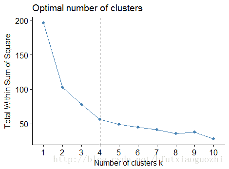
14.8 Elbow method to decide Optimal Number of Clusters (1)

set.seed(8)
wss <- function(k){return(kmeans(df, k, nstart = 25)$tot.withinss)
}k_values <- 1:15wss_values <- purrr::map_dbl(k_values, wss)plot(x = k_values, y = wss_values, type = "b", frame = F,xlab = "Number of clusters K",ylab = "Total within-clusters sum of square")

在这里插入图片描述

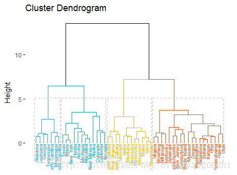
14.9 Hierarchical Clustering

hac_output <- hclust(dist(USArrests, method = "euclidean"), method = "complete")
plot(hac_output)

在这里插入图片描述

14.10 Ouput Desirable Number of Clusters After Modeling

> for (i in 1:length(hac_cut)){
+     if(hac_cut[i] != km_output$cluster[i]) print(names(hac_cut)[i])
+ }
[1] "Colorado"
[1] "Delaware"
[1] "Georgia"
[1] "Missouri"
[1] "Tennessee"
[1] "Texas"

15.Demo(2)

15.1 数据准备

#install.packages("ggplot2")
#install.packages("factoextra")
#载入包
library(factoextra)
# 载入数据
data("USArrests") 
# 数据进行标准化
df <- scale(USArrests) 
# 查看数据的前五行
head(df, n = 5)Murder   Assault   UrbanPop         Rape
Alabama    1.24256408 0.7828393 -0.5209066 -0.003416473
Alaska     0.50786248 1.1068225 -1.2117642  2.484202941
Arizona    0.07163341 1.4788032  0.9989801  1.042878388
Arkansas   0.23234938 0.2308680 -1.0735927 -0.184916602
California 0.27826823 1.2628144  1.7589234  2.067820292#确定最佳聚类数目
fviz_nbclust(df, kmeans, method = "wss") + geom_vline(xintercept = 4, linetype = 2)

æœ€ä½³èšç±»æ•°ç›®

15.2 K-means聚类

#从指标上看，选择坡度变化不明显的点最为最佳聚类数目。可以初步认为聚为四类最合适。
#设置随机数种子，保证实验的可重复进行
set.seed(123)
#利用k-mean是进行聚类
km_result <- kmeans(df, 4, nstart = 24)
#查看聚类的一些结果
print(km_result)
#提取类标签并且与原始数据进行合并
dd <- cbind(USArrests, cluster = km_result$cluster)
head(dd)Murder Assault UrbanPop Rape cluster
Alabama      13.2     236       58 21.2       4
Alaska       10.0     263       48 44.5       3
Arizona       8.1     294       80 31.0       3
Arkansas      8.8     190       50 19.5       4
California    9.0     276       91 40.6       3
Colorado      7.9     204       78 38.7       3#查看每一类的数目
table(dd$cluster)1  2  3  4 
13 16 13  8 
#进行可视化展示
fviz_cluster(km_result, data = df,palette = c("#2E9FDF", "#00AFBB", "#E7B800", "#FC4E07"),ellipse.type = "euclid",star.plot = TRUE, repel = TRUE,ggtheme = theme_minimal()
)

èšç±»æ•ˆæžœå›¾

15.3 层次聚类

#先求样本之间两两相似性
result <- dist(df, method = "euclidean")#产生层次结构
result_hc <- hclust(d = result, method = "ward.D2")#进行初步展示
fviz_dend(result_hc, cex = 0.6)

å±‚æ¬¡ç»“æž„å›¾

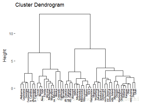
fviz_dend(result_hc, k = 4, cex = 0.5, k_colors = c("#2E9FDF", "#00AFBB", "#E7B800", "#FC4E07"),color_labels_by_k = TRUE, rect = TRUE          
)

å±‚æ¬¡èšç±»æ•ˆæžœå›¾

15.4 All code

#load library
library(ggplot2)
library(factoextra)# load data
data("USArrests") # Data standardization
df <- scale(USArrests) # Top 10 rows of view data
head(df, n = 10)# Determining the optimal number of clusters
fviz_nbclust(df, kmeans, method = "wss") + geom_vline(xintercept = 4, linetype = 2)# From the point of view of the index, the best number of 
# clustering is to select the points whose gradient changes are not obvious. 
# It is preliminarily considered that it is most appropriate to divide into four categories.# Setting up random number seeds to ensure the repeatability of the experiment
set.seed(123)# Clustering by K-means
km_result <- kmeans(df, 4, nstart = 24)# Look at some of the results of clustering
print(km_result)# Extract class labels and merge them with the original data
dd <- cbind(USArrests, cluster = km_result$cluster)
head(dd)# View the number of each category
table(dd$cluster)# Visual display
fviz_cluster(km_result, data = df,palette = c("#2E9FDF", "#00AFBB", "#E7B800", "#FC4E07"),ellipse.type = "euclid",star.plot = TRUE, repel = TRUE,ggtheme = theme_minimal()
)# Seek the similarity between two samples
result <- dist(df, method = "euclidean")# Generating hierarchy
result_hc <- hclust(d = result, method = "ward.D2")# preliminary dispaly
fviz_dend(result_hc, cex = 0.6)# According to this graph, it is convenient to determine the suitable
# grouping into several categories, such as we grouped into four categories 
# and displayed visually.fviz_dend(result_hc, k = 4, cex = 0.5, k_colors = c("#2E9FDF", "#00AFBB", "#E7B800", "#FC4E07"),color_labels_by_k = TRUE, rect = TRUE          
)

16.Homework

Option 1:Pick a dataset of your choice, apply both K-means and HAC algorithms to identify the underlying cluster structures and compare the differene between two outputs (if you are using a labeled dataset, you can also evaluate the performance of the cluster assignments by comparing them to the true class labels)
Submit your R codes with the cluster assignment outputs.Option 2:Identify a successful real world application of cluster analysis algorithm and discuss how it works. Please include a discussion of your understanding of clustering model, and how clustering model helps discover hidden data patterns for the application. The application could be in any kind of industries: banking, insurance, education, public administration, technology, healthcare management, etc.
Submit your essay which should be no less than 300 words