在这里插入图片描述

关注微信公众号：脑机接口研习社
了解脑机接口最近进展

系列文章目录

Python专栏 | 脑电图和脑磁图(EEG/MEG)的数据分析方法之载入数据

Python专栏 | MNE脑电数据(EEG/MEG)可视化

Python专栏 | MNE数据预处理方法——独立成分分析

持续更新中……

文章目录

系列文章目录
举个例子
- 1. 载入数据（Loading data）
- 2. Visualizing the artifacts
- 3. Filtering to remove slow drifts
- 4. Fitting and plotting the ICA solution
总结

举个例子

独立成分分析（ICA）的一个应用例子是利用ICA消除伪影（artifacts）。

伪影是医学影像领域中的专业术语。伪影可以定义为图像中在视场（FOV）里歪曲物体的任何特征。所有MRI图像都包含一些伪影，它们的识别对于避免误诊和获取诊断图像很重要。被试的运动（例如呼吸，肠蠕动、心脏跳动、眼皮跳动等正常的生理活动）、设备、软件等因素均会引起伪影。

下面讲解如何利用ICA消除伪影。

1. 载入数据（Loading data）

关于在MNE里载入数据的代码解释可点击查看下面这篇文章：

脑电图和脑磁图(EEG/MEG)的数据分析方法之载入数据

代码示例：

import os
import mne
from mne.preprocessing 
import (ICA, create_eog_epochs, create_ecg_epochs, corrmap)sample_data_folder = mne.datasets.sample.data_path()sample_data_raw_file = os.path.join(sample_data_folder, 'MEG', 'sample',                                    'sample_audvis_raw.fif')raw = mne.io.read_raw_fif(sample_data_raw_file)

输出结果：

Opening raw data file /home/circleci/mne_data/MNE-sample-data/MEG/sample/sample_audvis_raw.fif...    
Read a total of 3 projection items:        
PCA-v1 (1 x 102)  idle       PCA-v2 (1 x 102)  idle        
PCA-v3 (1 x 102)  idle    Range : 25800 ... 192599 =     42.956 ...   320.670 secs
Ready.

2. Visualizing the artifacts

让我们首先从可视化我们要修复的伪影开始。在已有数据集中，伪影是足够大的，可以很容易地在原始数据中看到：

代码示例：

#pick some channels that clearly show heartbeats and blinks
regexp = r'(MEG [12][45][123]1|EEG 00.)'artifact_picks = mne.pick_channels_regexp(raw.ch_names, regexp=regexp)raw.plot(order=artifact_picks, n_channels=len(artifact_picks),show_scrollbars=False)

输出结果：
在这里插入图片描述
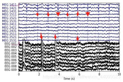
如上图所示，波段突起的部分（图上红色箭头部分）就是由于眼动或心脏跳动引起的运动性伪影（红色箭头为小编所加）。

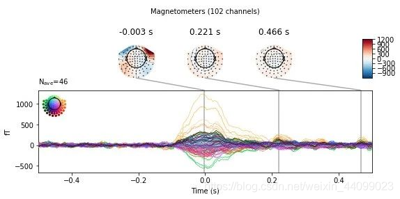
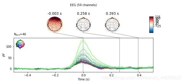
下面利用create_eog_epochs显示每个通道中的眼动伪影（ocular artifact），即将上图中的突起波段进行突出显示。

代码示例：

eog_evoked = create_eog_epochs(raw).average()eog_evoked.apply_baseline(baseline=(None, -0.2))eog_evoked.plot_joint()

Electrocardiogram (ECG）心电图
Electrooculogram (EOG) 眼电图

详细代码请参考：
https://mne.tools/stable/auto_tutorials/preprocessing/plot_10_preprocessing_overview.html#tut-artifact-overview

输出结果：
在这里插入图片描述

EOG channel index for this subject is: [375]
Filtering the data to remove DC offset to help distinguish blinks from saccades
Setting up band-pass filter from 1 - 10 Hz
FIR filter parameters
---------------------
Designing a two-pass forward and reverse, zero-phase, non-causal bandpass filter:
- Windowed frequency-domain design (firwin2) method
- Hann window
- Lower passband edge: 1.00
- Lower transition bandwidth: 0.50 Hz (-12 dB cutoff frequency: 0.75 Hz)
- Upper passband edge: 10.00 Hz
- Upper transition bandwidth: 0.50 Hz (-12 dB cutoff frequency: 10.25 Hz)
- Filter length: 6007 samples (10.001 sec)
Now detecting blinks and generating corresponding events
Found 46 significant peaks
Number of EOG events detected : 46
Not setting metadata
Not setting metadata
46 matching events found
No baseline correction applied
Created an SSP operator (subspace dimension = 3)
Loading data for 46 events and 601 original time points ...
C:\ProgramData\Anaconda3\lib\site-packages\mkl_fft\_numpy_fft.py:331: FutureWarning: Using a non-tuple sequence for multidimensional indexing is deprecated; use `arr[tuple(seq)]` instead of `arr[seq]`. In the future this will be interpreted as an array index, `arr[np.array(seq)]`, which will result either in an error or a different result.output = mkl_fft.rfft_numpy(a, n=n, axis=axis)
0 bad epochs dropped
Applying baseline correction (mode: mean)
Created an SSP operator (subspace dimension = 3)
3 projection items activated
SSP projectors applied...
Removing projector <Projection | PCA-v1, active : True, n_channels : 102>
Removing projector <Projection | PCA-v2, active : True, n_channels : 102>
Removing projector <Projection | PCA-v3, active : True, n_channels : 102>
Removing projector <Projection | PCA-v1, active : True, n_channels : 102>
Removing projector <Projection | PCA-v2, active : True, n_channels : 102>
Removing projector <Projection | PCA-v3, active : True, n_channels : 102>
<Figure size 576x302.4 with 7 Axes>,<Figure size 576x302.4 with 7 Axes>,<Figure size 576x302.4 with 7 Axes>

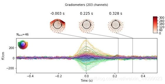
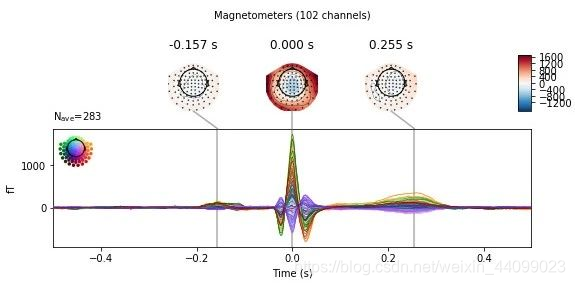
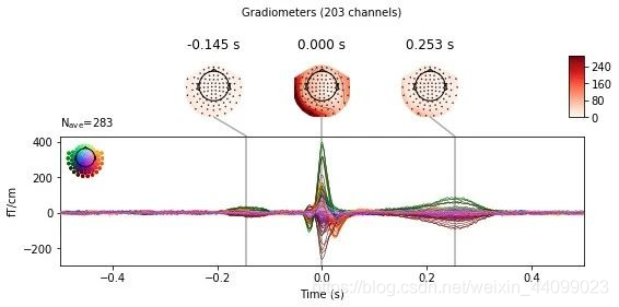
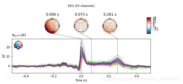
同样的道理，我们利用create_ecg_epochs来可视化心脏跳动伪影。

代码示例：

ecg_evoked = create_ecg_epochs(raw).average()
ecg_evoked.apply_baseline(baseline=(None, -0.2))
ecg_evoked.plot_joint()

输出结果：
在这里插入图片描述

Reconstructing ECG signal from Magnetometers
Setting up band-pass filter from 8 - 16 Hz
FIR filter parameters
---------------------
Designing a two-pass forward and reverse, zero-phase, non-causal bandpass filter:
- Windowed frequency-domain design (firwin2) method
- Hann window
- Lower passband edge: 8.00
- Lower transition bandwidth: 0.50 Hz (-12 dB cutoff frequency: 7.75 Hz)
- Upper passband edge: 16.00 Hz
- Upper transition bandwidth: 0.50 Hz (-12 dB cutoff frequency: 16.25 Hz)
- Filter length: 6007 samples (10.001 sec)
C:\ProgramData\Anaconda3\lib\site-packages\mkl_fft\_numpy_fft.py:331: FutureWarning: Using a non-tuple sequence for multidimensional indexing is deprecated; use `arr[tuple(seq)]` instead of `arr[seq]`. In the future this will be interpreted as an array index, `arr[np.array(seq)]`, which will result either in an error or a different result.output = mkl_fft.rfft_numpy(a, n=n, axis=axis)
Number of ECG events detected : 283 (average pulse 61 / min.)
Not setting metadata
Not setting metadata
283 matching events found
No baseline correction applied
Created an SSP operator (subspace dimension = 3)
Loading data for 283 events and 601 original time points ...
0 bad epochs dropped
Applying baseline correction (mode: mean)
Created an SSP operator (subspace dimension = 3)
3 projection items activated
SSP projectors applied...
Removing projector <Projection | PCA-v1, active : True, n_channels : 102>
Removing projector <Projection | PCA-v2, active : True, n_channels : 102>
Removing projector <Projection | PCA-v3, active : True, n_channels : 102>
Removing projector <Projection | PCA-v1, active : True, n_channels : 102>
Removing projector <Projection | PCA-v2, active : True, n_channels : 102>
Removing projector <Projection | PCA-v3, active : True, n_channels : 102>[<Figure size 576x302.4 with 7 Axes>,<Figure size 576x302.4 with 7 Axes>,<Figure size 576x302.4 with 7 Axes>]

3. Filtering to remove slow drifts

在运行ICA之前，比较重要的一个步骤是对数据进行滤波以消除低频漂移（low-frequency drifts），因为低频漂移可能会对ICA的拟合质量产生负面影响。

慢的漂移（slow drifts）是比较棘手的，因为它们会降低独立来源的独立性（independency）。

例如在上一篇提到的“鸡尾酒宴会问题”。详见：

MNE数据预处理方法——独立成分分析

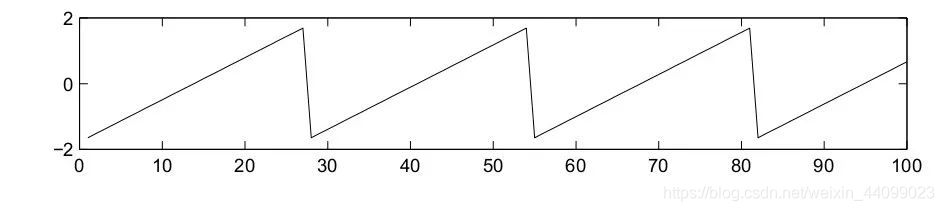
我们想要还原的信号是下图 s，从图中可以看出信号波动明显，信号源非常具有独立性。
在这里插入图片描述

但是我们实际得到的信号是下图 x，中间由于存在许多slow drifts，所以信号源丧失了其独立性（红色箭头为小编所加）。
在这里插入图片描述

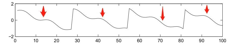
低频漂移的存在使得算法很难找到准确的ICA解决方案（ICA solution）。

这里建议使用截止频率为1Hz的低通滤波器。

由于滤波是线性操作，因此可以将已过滤信号中的ICA解决方案，应用于未过滤的信号。

更多信息请参见：https://doi.org/10.1109/EMBC.2015.7319296

所以我们将保留未过滤的Raw对象的副本，以便我们可以稍后对其应用ICA解决方案。

代码示例：

#过滤低频漂移
filt_raw = raw.copy() #创建副本
filt_raw.load_data().filter(l_freq=1., h_freq=None)

输出结果：

Reading 0 ... 166799  =      0.000 ...   277.714 secs...
Filtering raw data in 1 contiguous segment
Setting up high-pass filter at 1 Hz
FIR filter parameters
---------------------
Designing a one-pass, zero-phase, non-causal highpass filter:
- Windowed time-domain design (firwin) method
- Hamming window with 0.0194 passband ripple and 53 dB stopband attenuation
- Lower passband edge: 1.00
- Lower transition bandwidth: 1.00 Hz (-6 dB cutoff frequency: 0.50 Hz)
- Filter length: 1983 samples (3.302 sec)

4. Fitting and plotting the ICA solution

现在，我们准备设置并安装ICA。
在这里插入图片描述
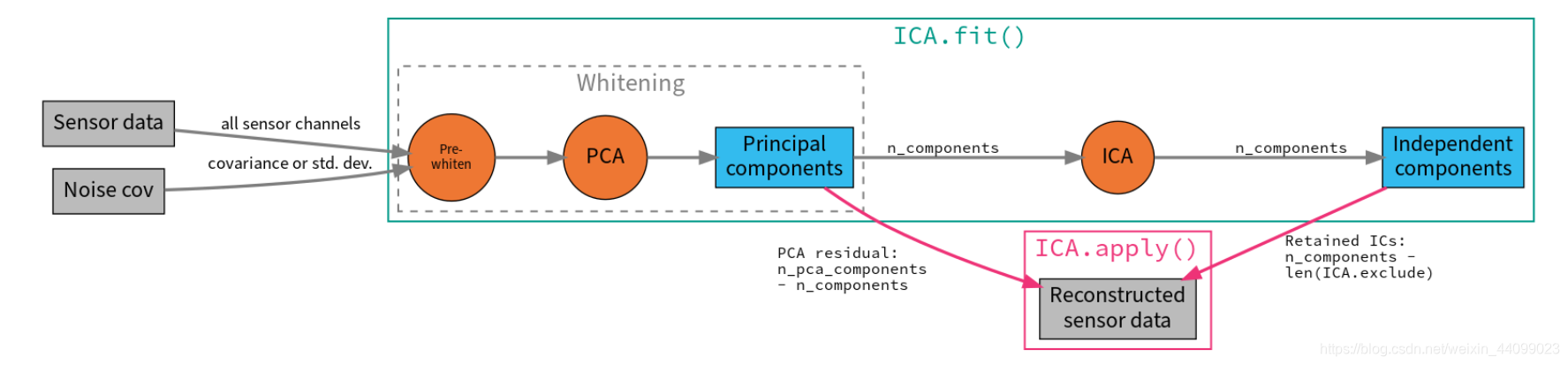
▲点击图片可查看大图

既然我们通过观察原始数据，知道EOG和ECG的伪影相当显著，所以我们希望这些伪影在PCA分解的前几个维度中捕获。

我们可能不需要大量的分量（components）就可以很好地完成分解伪影的工作。通常情况下，最好n_components设置的大一些，会分解的较为精准。

n_components是需要不断尝试和测试，来最终确定到底设置成多少。

第一次尝试，我们将以n_components = 15来运行ICA。考虑到我们的Raw data里有超过300个以上的通道，故将n_components设置成15实际上偏小了，但是这样可以运行的比较快。

ICA拟合（ICA.fit）不是确定性的，例如，components在不同的运行过程中可能会出现符号翻转（sign flip），或者不一定总是以相同的顺序返回。因此我们还将指定一个随机种子（random seed），以便每次都能获得相同的结果。

代码示例：

ica = ICA(n_components=15, random_state=97)
ica.fit(filt_raw)

输出结果：

Fitting ICA to data using 364 channels (please be patient, this may take a while)
Selecting by number: 15 components
Fitting ICA took 8.9s.
<ICA | raw data decomposition, fit (fastica): 166800 samples, 15 components, channels used: "mag"; "grad"; "eeg">

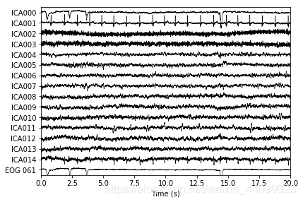
接着，我们可以通过查看独立成分（Independent Components, ICs），来看它们捕获了什么。

plot_sources将显示ICs的时间序列。

代码示例：

#ICA结果的可视化呈现
filt_raw.load_data()
ica.plot_sources(filt_raw, show_scrollbars=False)

输出结果：
在这里插入图片描述

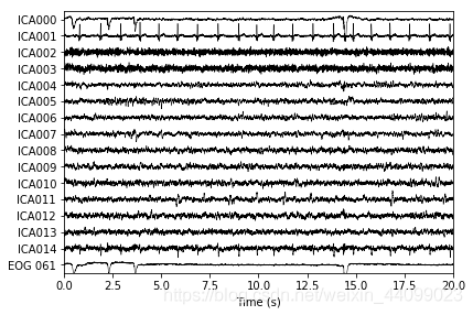
Creating RawArray with float64 data, n_channels=16, n_times=166800Range : 25800 ... 192599 =     42.956 ...   320.670 secs
Ready.

Note：
在对plot_sources的调用中，我们可以使用未经过滤的原始Raw对象。

代码示例：

raw.load_data()
ica.plot_sources(raw, show_scrollbars=False)

输出结果：
在这里插入图片描述

Creating RawArray with float64 data, n_channels=16, n_times=166800Range : 25800 ... 192599 =     42.956 ...   320.670 secs
Ready.

由上图可知，第一个分量（ICA000）很好地捕获了EOG 061信号，第二个组件（ICA001）看起来很像心跳。

P.S.有关在视觉上识别独立成分IC的更多信息，EEGLAB教程是一个很好的参考资料。https://labeling.ucsd.edu/tutorial/labels

我们还可以使用plot_components可视化每个组件的头皮区域（scalp field distribution）分布。

代码示例：

ica.plot_components()

输出结果：

在这里插入图片描述

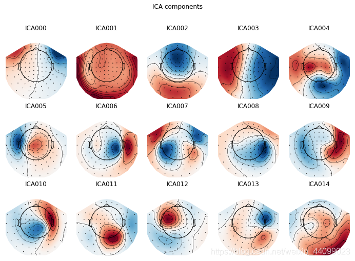
在上面的图中，很明显地可以看出，哪些IC正在捕获被试的EOG和ECG伪影。

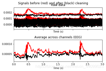
同时，也有其他的可视化方案。我们还可以使用plot_overlay绘制原始信号与排除了伪影的重构信号的对比图。

代码示例：

# blinks 
ica.plot_overlay(raw, exclude=[0], picks='eeg')
#选择EEG，是因为EEG更容易监测到眨眼活动。exclude=[0]中的0是指上面的ICA000。# heartbeats 
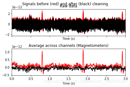
ica.plot_overlay(raw, exclude=[1], picks='mag')
#选择MAG，是因为MAG更容易监测到心脏跳动。exclude=[1]中的1是指上面的ICA001。

输出结果：
在这里插入图片描述

Applying ICA to Raw instanceTransforming to ICA space (15 components)Zeroing out 1 ICA componentProjecting back using 364 PCA componentsApplying ICA to Raw instanceTransforming to ICA space (15 components)Zeroing out 1 ICA componentProjecting back using 364 PCA components

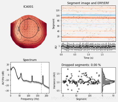
我们还可以使用plot_properties绘制每个IC的一些诊断信息：

代码示例：

ica.plot_properties(raw, picks=[0, 1])
#选择ICA000和ICA001

输出结果：
在这里插入图片描述

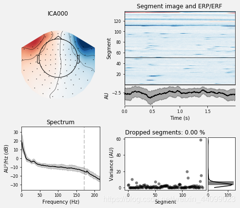
Using multitaper spectrum estimation with 7 DPSS windows
Not setting metadata
Not setting metadata
138 matching events found
No baseline correction applied
0 projection items activated
0 bad epochs dropped
Not setting metadata
Not setting metadata
138 matching events found
No baseline correction applied
0 projection items activated
0 bad epochs dropped

总结

今天用到的代码总结：

#载入数据
import os
import numpy as np
import mne
from mne.preprocessing import (ICA, create_eog_epochs, create_ecg_epochs,corrmap)sample_data_folder = mne.datasets.sample.data_path()
sample_data_raw_file = os.path.join(sample_data_folder, 'MEG', 'sample','sample_audvis_raw.fif')
raw = mne.io.read_raw_fif(sample_data_raw_file)#raw.crop(tmax=60.) #取60s的数据#可视化伪影
# pick some channels that clearly show heartbeats and blinks
regexp = r'(MEG [12][45][123]1|EEG 00.)'
artifact_picks = mne.pick_channels_regexp(raw.ch_names, regexp=regexp)
raw.plot(order=artifact_picks, n_channels=len(artifact_picks),show_scrollbars=False)#利用create_eog_epochs显示每个通道中的眼动伪影（ocular artifact），
#详细代码参考：https://mne.tools/stable/auto_tutorials/preprocessing/plot_10_preprocessing_overview.html#tut-artifact-overview
eog_evoked = create_eog_epochs(raw).average()
eog_evoked.apply_baseline(baseline=(None, -0.2))
eog_evoked.plot_joint()
#Electrocardiogram (ECG）心电图；Electrooculogram (EOG) 眼电图#同样的道理，我们利用create_ecg_epochs来可视化心脏跳动伪影
ecg_evoked = create_ecg_epochs(raw).average()
ecg_evoked.apply_baseline(baseline=(None, -0.2))
ecg_evoked.plot_joint()#过滤低频漂移
filt_raw = raw.copy() #创建副本
filt_raw.load_data().filter(l_freq=1., h_freq=None)#ICA拟合
ica = ICA(n_components=15, random_state=97)
ica.fit(filt_raw)#ICA结果的可视化呈现
filt_raw.load_data()
ica.plot_sources(filt_raw, show_scrollbars=False)#Note：在对plot_sources的调用中，我们也可以将ica应用在未经过滤的原始Raw对象上。
raw.load_data()
ica.plot_sources(raw, show_scrollbars=False)#使用plot_components可视化每个组件的头皮区域（scalp field distribution）分布。 
ica.plot_components()#可以使用plot_overlay绘制原始信号与排除了伪影的重构信号的对比图。
# blinks 眨眼伪影
ica.plot_overlay(raw, exclude=[0], picks='eeg')
#选择EEG，是因为EEG更容易监测到眨眼活动。exclude=[0]中的0是指上面的ICA000。# heartbeats 心动伪影
ica.plot_overlay(raw, exclude=[1], picks='mag')
#选择MAG，是因为MAG更容易监测到心脏跳动。exclude=[1]中的0是指上面的ICA001。#我们还可以使用plot_properties绘制每个IC的一些诊断信息：
ica.plot_properties(raw, picks=[0, 1])#选择ICA000和ICA001