本案例是kaggle共享单车的比赛案例,先对数据集介绍
Instant 记录号
Dteday:日期
Season:季节 1=春天 2=夏天 3=秋天 4=冬天
yr:年份,(0: 2011, 1:2012)
mnth:月份( 1 to 12)
hr:小时 (0 to 23)
holiday:是否是节假日
weekday:星期中的哪天,取值为 0~6
workingday:是否工作日 1=工作日 (非周末和节假日)0=周末
weathersit:天气 1:晴天,多云 2:雾天,阴天 3:小雪,小雨 4:大雨,大雪,大雾
temp:气温摄氏度
atemp:体感温度
hum:湿度
windspeed:风速
casual:非注册用户个数(非会员)
registered:注册用户个数(会员)
cnt:给定日期(天)时间(每小时)总租车人数,响应变量 y
关于线性回归知识请回顾往期两篇文章:
线性回归之原理介绍
线性回归建模思路与模型诊断(附代码)
下面直接上代码操作。
1.导入相关模块
import pandas as pd
import numpy as np
import seaborn as sns
from scipy import stats
import matplotlib.pyplot as pltfrom jupyterthemes import jtplot
jtplot.style(theme='onedork') #选择一个绘图主题
jtplot.style(ticks=True, grid=False, figsize=(6,4))plt.rcParams['font.sans-serif']=['SimHei']
plt.rcParams['axes.unicode_minus']=False
2.加载数据并作描述性统计分析
data = pd.read_excel(r'D:\MLearn\共享单车\共享单车.xlsx')for i in ['season','yr','mnth','holiday','weekday','workingday','weathersit']:data[i] = data[i].astype(object) #声明离散型变量data.drop(['instant','dteday','casual','registered'],axis=1).describe(include='object')des = data.drop(['instant','casual','cnt','registered'],axis=1).describe().T
des['极差'] = des['max'] - des['min']
des['离散系数'] = des['std']/des['mean']
des.T.round(decimals=3)
观察结果:
离散型变量一共7个:季节、年份、月份、是否节假日、是否周末、是否工作日和天气
数据无缺失,都是731条数据记录。
连续型变量有4个,气温摄氏度(temp),体感温度(atemp),湿度(hum)和风速(windspeed)
从数据集中趋势看,中位数与均值基本持平,说明数据分布比较集中,
从数据离散程度看,湿度的变异程度最大,但离散系数最低,波动幅度最低;而风速的变异程度低,但波动幅度大。
3.对目标变量进行正态性检验
from scipy.stats import norm, skewa = data['cnt']sns.distplot(a, fit=norm)
(mu, sigma) = norm.fit(a)
print(mu, sigma)
print('Kurtosis: %f' % a.kurt())
print('Skewness: %f' % a.skew())fig = plt.figure()
res = stats.probplot(a, plot=plt)
plt.show()
结果如下:
拟合的均值为4500,方差1935。蓝色线不完全分布在红色上,峰度值为-0.8,偏度-0.04,表明数据呈现轻微低峰态的左偏分布。
再研究一下目标变量:看看时间跟租赁量的走势图:
data['year_month'] = data.dteday.dt.strftime('%Y-%m') #年月日转换为年月# 做每天租赁散点图和每月均值
group_month = data.groupby('year_month')['cnt'].mean()
group_month.index = pd.to_datetime(group_month.index)
plt.figure(figsize=(16,5))
plt.plot(data.dteday, data.cnt, '-', color = 'b', label = '每天租赁数量', alpha=0.5)
plt.plot(group_month.index, group_month.values, '-o', color='orange', label = '每月租赁数量均值')
plt.legend()
plt.show()
1.共享单车的租赁情况2012年整体比2011年有所增长;
2.租赁数量随月份波动且每年波动幅度相似;
3.有很多局部波峰波谷值且2012年波动情况比2011年大
4.对影响租赁量因素做整体探索
sns.pairplot(data ,x_vars=['holiday','workingday','weathersit','season','weekday', 'temp','atemp','hum','windspeed'] ,y_vars=['casual','registered','cnt'] , plot_kws={'alpha': 0.5})plt.show()结果如下,就是变量与目标的散点图分布:
1.会员在工作日出行量多,非工作日少,非会员则相反;
2.无论是会员还是非会员,节假日出行量多于非节假日;
3.租赁数量随天气等级上升而减少;
4.一季度出行量低于其他季度出行量
5.会员在星期一~星期五的出行量多于周六、周日,而非会员相反
6.租赁数量随风速增大而减少;
7.温度、湿度对非会员影响比较大,对会员影响较小
8.总体租赁量随着温度升高而升高
5.探索特征与目标之间的关系
对于离散变量,列举季节、月份对目标的影响,其余变量同理操作。
sns.violinplot(data=data[['season','cnt']],x="season",y="cnt")
plt.show()
能看出来每个季节骑行量的分布不同 barplot利用矩阵条的高度反映数值变量的集中趋势
fig,ax = plt.subplots()
sns.barplot(data=data[['mnth', 'cnt']], x="mnth",y="cnt")
ax.set(title="Monthly distribution of counts")
plt.show()
可以看出,一年12月份,单车投放量先上升后下降,峰值出现再6~8月份
对于连续变量,由于变量不多,直接给出相关关系图查看:
corrmatt = data[['temp','atemp','hum','windspeed','cnt']].corr()
plt.subplots(figsize=(6,4))
mask = np.array(corrmatt)
mask[np.tril_indices_from(mask)] = False
heatmap = sns.heatmap(corrmatt,annot=True,mask=mask,cmap="Blues")
plt.show()
1.气温摄氏度、体感温度与骑行量的相关性大于0.5,而湿度、风速与骑行量的相关性很低
2.气温摄氏度与体感温度的相关性高达0.99
再进一步挖掘,
#按温度取租赁额平均值
data['temp_group'] = pd.cut(data['temp'], bins=[0.05*i for i in range(21)],right=False)
temp_rentals = data.groupby(['temp_group'], as_index=True).agg({'casual':'mean', 'registered':'mean','cnt':'mean'})
temp_rentals .plot(title = 'The average number of rentals initiated per hour changes with the temperature')
# plt.xticks(rotation=45)
plt.show()
随着温度的上升,租赁量也增加,在0.7附近达到最高峰,之后随着温度升高,租赁量开始缓慢下降
6.假设检验
对于双样本,这里展示年份对目标影响的显著性检验,其余操作同理。
arg = []
li = [2011,2012]
for i in data['yr'].value_counts().index:arg.append(data[data['yr'] == i]['cnt'])sns.boxplot(data=arg,palette='deep') #箱线图,设置6种颜色;调色板
plt.show()# stats.f_oneway(*arg)
des = data['cnt'].groupby(data['yr']).describe()
des['cov'] = des['std']/des['mean']
des
箱线图如下图:
可见2011和2012骑行量均值有很大差别,下面进一步从统计学上验证该差异显著
#方差齐性检验 H0:两组数据方差相同
year2011 = data[data['yr'] == 0]['cnt']
year2012 = data[data['yr'] == 1]['cnt']
leveneTestRes = stats.levene(year2011, year2012, center='median')
print('w-value=%6.4f, p-value=%6.4f' %leveneTestRes)
检验结果:
p小于0.05,拒绝原假设,即两组数据方差不相同,有显著差异。因此不能采用t检验,要采取大样本u检验
from scipy.stats import normdes['S'] = des['std']**2  #总体方差的无偏估计,describe内置的std分母是n-1
des[['count','mean','S']]
u = (des['mean'][0]-des['mean'][1])/np.sqrt(np.sum(des['S']/des['count'])) #检验统计量
p = norm.cdf(u,0,1) #概率密度函数在 负无穷 到 u上的积分,也就是概率print('u-value=%6.4f, p-value=%6.4f' % (u,2*p)) #双侧检验,乘以2
检验结果p远小于0.05,因此可以认为均值有显著差异。
对于多样本检验,也就是要进行方差分析,这里以季节为例:
arg = []
li = []
for i in data['season'].value_counts().index:li.append(i)arg.append(data[data['season'] == i]['cnt'])sns.set_style('whitegrid') #箱线图,观察异常值
jtplot.style(theme='onedork') #选择一个绘图主题
jtplot.style(ticks=True, grid=False, figsize=(10, 8))
plt.rcParams['font.sans-serif']=['SimHei']
plt.rcParams['axes.unicode_minus']=Falsesns.boxplot(data=arg,palette='deep') #箱线图,设置6种颜色;调色板
# plt.xticks(range(16),li,rotation=90)
plt.show()print('单因素方差分析:',stats.f_oneway(*arg))
箱线图与检验结果如下:
p值远小于0.05,因此,季节对均值有显著影响。
注:除了单因素方差分析,我们还有多因素方差分析,就是考虑两个变量交互作用的影响,以下代码实现了这个过程(本节的建模不考虑这种影响)
import statsmodels.formula.api as smf
import statsmodels.api as smli = ['season','mnth','weathersit']for n,i in enumerate(li):for j in li[n+1:]:# smf:最小二乘法,构建线性回归模型anal = smf.ols('cnt ~ C({}) + C({}) + C({})*C({})'.format(i,j,i,j), data=data).fit()# anova_lm:多因素方差分析re = sm.stats.anova_lm(anal)re = pd.DataFrame(re)if list(re['PR(>F)'])[2] > 0.01:print('{}和{}交互作用对单车投放量影响无显著差别,考虑无交互作用的情况'.format(i,j))#考虑无交互作用的方差分析anal = smf.ols('cnt ~ C({}) + C({})'.format(i,j), data=data).fit()# anova_lm:多因素方差分析re = sm.stats.anova_lm(anal)else:print('{}和{}交互作用对单车投放量影响有差别'.format(i,j))print(re)print('********************************************************')
7.特征工程
基于前面步骤的分析,我们可以筛选、构造一些特征。然后做一定的特征工程处理,离散变量需要连续化,一般采用one-hot编码(独热编码)
feature_col = ['season','mnth','weathersit','yr']
for feature in feature_col:data[feature] = data[feature].astype('object')season_di = {1:'spring',2:'summer',3:'autumn',4:'winter'}
month_di = {1:'Jan',2:'Feb',3:'Mar',4:'Apr',5:'May',6:'Jun',7:'Jul',8:'Aug',9:'Sep',10:'Oct',11:'Nov',12:'Dec'}
weather_di = {1:'sunny',2:'fog',3:'rain',4:'snow'}
year_di = {0:2011,1:2012}data_cat = data[feature_col]
data_cat['season'] = data_cat['season'].replace(season_di)
data_cat['mnth'] = data_cat['mnth'].replace(month_di)
data_cat['weathersit'] = data_cat['weathersit'].replace(weather_di)
data_cat['yr'] = data_cat['yr'].replace(year_di).astype(object)data_cat = pd.get_dummies(data_cat) #独热编码
如有需要,还要进行归一化处理,以后会专门出一起关于归一化的问题,利用下面代码可以进行归一化处理。本次建模做了均值标准差归一化处理。
from sklearn.preprocessing import MinMaxScaler #线性函数归一化
from sklearn.preprocessing import StandardScaler #均值与标准差归一化
8.模型建立与调参
采用L2正则进行建模,利用网格搜索寻找最优超参数,本次建模采取r2评价指标(也就是可决系数)
from sklearn.linear_model import RidgeCV
from sklearn.linear_model import LassoCV
from sklearn.model_selection import GridSearchCV
from sklearn.model_selection import train_test_split
from sklearn.metrics import make_scorer,log_loss,r2_score,mean_squared_error #评价指标,损失函数
切分训练测试集,这里二八分:
X_train,X_test,y_train,y_test = train_test_split(X,y,test_size=0.2,random_state=0)首先,随机挑选几个超参数:
alphas= [0.1,1,5,10]model = RidgeCV(alphas=alphas,fit_intercept=True,scoring=None, cv=5)model.fit(X_train,y_train)y_pred = model.predict(X_test)
# print('train of mean_squared_error is:',mean_squared_error(y_train,model.predict(X_train)))
# print('test of mean_squared_error is:',mean_squared_error(y_test,y_pred))
print(model.alpha_)
print('train of R2 is:',r2_score(y_train,model.predict(X_train)))
print('test of R2 is:',r2_score(y_test,y_pred))
结果如下:
然后从1~10之间利用网格搜索逐步寻找最佳的超参数,笔者一共迭代了4次,最终找到了合适的超参数C=4.213
第一轮迭代:
alphas= np.linspace(1,10,21)
model = RidgeCV(alphas=alphas,fit_intercept=False,scoring=None, cv=5)
model.fit(X_train,y_train)
y_pred = model.predict(X_test)
print(model.alpha_)
print('train of R2 is:',r2_score(y_train,model.predict(X_train)))
print('test of R2 is:',r2_score(y_test,y_pred))
第二轮迭代:
alphas= np.linspace(3.7 ,4.6,21)
model = RidgeCV(alphas=alphas,fit_intercept=False,scoring=None, cv=5)
model.fit(X_train,y_train)
y_pred = model.predict(X_test)
print(model.alpha_)
print('train of R2 is:',r2_score(y_train,model.predict(X_train)))
print('test of R2 is:',r2_score(y_test,y_pred))
第三轮迭代:
alphas= np.linspace(4.15 ,4.24,21)
model = RidgeCV(alphas=alphas,fit_intercept=False,scoring=None, cv=5)
model.fit(X_train,y_train)
y_pred = model.predict(X_test)
print(model.alpha_)
print('train of R2 is:',r2_score(y_train,model.predict(X_train)))
print('test of R2 is:',r2_score(y_test,y_pred))
第四轮迭代:
alphas= np.linspace(4.2085 ,4.2175,21)
model = RidgeCV(alphas=alphas,fit_intercept=False,scoring=None, cv=5)
model.fit(X_train,y_train)
y_pred = model.predict(X_test)
print(model.alpha_)
print('train of R2 is:',r2_score(y_train,model.predict(X_train)))
print('test of R2 is:',r2_score(y_test,y_pred))
可见,第四轮后,训练集和测试集的R2没有变化了,且两者都是0.8369.说明超参数已经最优了。
9.诊断方差与偏差
绘制学习曲线和验证曲线去观察偏差与方差,先来看学习曲线:
from sklearn.linear_model import Ridge
from sklearn.model_selection import learning_curve #学习曲线,方差与偏高的诊断
from sklearn.model_selection import ShuffleSplitcv = ShuffleSplit(n_splits=10, test_size=0.3, random_state=0)li = np.linspace(0.1,1,10)
train_sizes, train_loss, test_loss = learning_curve(Ridge(alpha=4.213,fit_intercept=False,random_state=0),X, y, cv=cv, scoring ='r2',train_sizes=li)train_score = np.mean(train_loss,axis=1)
test_score = np.mean(test_loss,axis=1)
plt.figure()
plt.plot(li,train_score,'o-',color = 'b',label = 'Training')
plt.plot(li,test_score,'o-',color = 'r',label = 'Testing')
# plt.plot(li,[0.115 for i in range(len(li))],'--',color = 'g',label = 'Desired')
plt.legend(loc='best')
plt.title('learning curve')
plt.xlabel('traing set size')
plt.ylabel('R2')
plt.show()
注:这里做了10折交叉验证,利用ShuffleSplit模块实现的,举一个例子解释它的工作原理
假设参数输入如下:
ShuffleSplit(n_splits=5, test_size=0.2, random_state=0)
利用20%数据集作为验证集,80%作为训练集,对同一份数据集做重复5次这样的过程。然后训练时,5次采样都建模,最后用采样的5次验证集的平均结果作为最终的输出结果。
注意,这里与我们常说的交叉验证不太一样,因为每次的验证集样本可能有重复的,而我们的交叉验证的每次的测试集都是不一样的。源码也给出了解释。
严格的交叉验证是下面这样的(估计大家这张图不陌生,利用模块kflod可以实现)
好了,回到正题,我们解读我们模型的学习曲线:
解读学习曲线:一开始,训练集样本只有10%的时候,模型严重过拟合,训练集R2表现比测试集的好了很多,随着样本增加,观察到,训练集R2指标降低,测试集上升,模型过拟合效果逐渐被改善,当用完所有样本进行训练时,二者的R2已经非常接近了,模型拟合效果良好。
再来看验证曲线的表现,
from sklearn.model_selection import validation_curvecv = ShuffleSplit(n_splits=10, test_size=0.3, random_state=0)
li = np.linspace(0.1,10,21)train_loss, test_loss = validation_curve(Ridge(fit_intercept=False,random_state=0),X, y, cv=cv,scoring ='r2',param_name='alpha',param_range=li)train_score = np.mean(train_loss,axis=1)
test_score = np.mean(test_loss,axis=1)
plt.figure()
plt.plot(li,train_score,'o-',color = 'b',label = 'Training')
plt.plot(li,test_score,'o-',color = 'r',label = 'Testing')
plt.legend(loc='best')
plt.title('validation curve')
plt.xlabel('value of C')
plt.ylabel('R2')
plt.show()
刚开始看起来,好像训练集测试集的R2相差很大,但是我们注意到纵坐标的刻度,其实误差已经在0.01范围了。解读这个验证曲线:
一开始,对超参数惩罚很低时,模型过拟合,随着惩罚的增加,训练集效果一直下降,而测试集先上升后下降,说明模型过拟合效果减轻,当达到一定程度后,继续加大惩罚,训练集和测试集效果都下降。这就说明超参数的调节对于最优模型的选择是多么的重要了。
最后我们看看拟合出来特征系数:
# Plot important coefficients
coefs = pd.Series(model.coef_, index = X_train.columns)
print("Ridge picked " + str(sum(coefs != 0)) + " features")#系数值变量排序
imp_coefs = pd.concat([coefs.sort_values()])
imp_coefs.plot(kind = "barh")
plt.title("Coefficients in the OLS Model")
plt.show()关于回归诊断更多的内容,比如残差独立性检验等。这里不再展示了,代码已在另外一篇文章给出。
关于线性回归的建模实操案例分享到这。最后强调一句,实际业务的建模,如果采用R2作为评价指标,达到0.4以上已经是一个不错的模型了。具体情况还需结合业务进一步分析。