文章目录

第五章多视图几何
- 5.1 外极几何
- - 5.1.1 一个简单的数据集
  - 5.1.2 用Matplotlib绘制三维数据
  - 5.1.3 计算F：八点法
  - 5.1.4 外极点和外极线
- 5.2 照相机和三维结构的计算
- - 5.2.1 三角剖分
  - 5.2.2 由三维点计算照相机矩阵
  - 5.2.3 由基础矩阵计算照相机矩阵
- 5.3 多视图重建
- - 5.3.1 稳健估计基础矩阵
  - 5.3.2 三维重建示例
- sfm.py

第五章多视图几何

本章主要讲如何通过处理多个视图以及如何利用多个视图的几何关系来恢复照相机位置信息和三维结构。

通过不同视点拍摄的图像，可以利用特征匹配来计算出三维场景点以及照相机位置。

5.1 外极几何

理论知识：

多视图几何是利用在不同视点所拍摄图像间的关系，来研究照相机之间或者特征之间关系的一门科学。本章使用兴趣点特征。

多视图几何中最重要的内容是双视图几何，本章使用的是双视图几何。

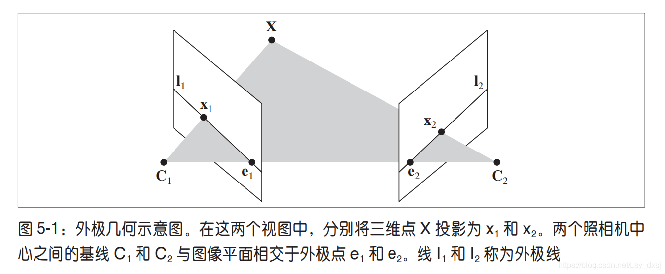
如果有一个场景的两个视图以及视图中的对应图像点，那么根据照相机间的空间相对位置关系、照相机的性质以及三维场景点的位置，可以得到对这些图像点的一些几何关系约束。我们通过外极几何来描述这些几何关系。

没有关于照相机的先验知识，会出现固有二义性。

一个文法存在某个句子对应两棵不同的语法树，则称这个文法是二义的。也就是该句子有两个不同的最左（最右）推导。

因为三维场景点 $X$ 经过4×4的单应性矩阵 $H$ 变换为 $H X$ 后，则 $H X$ 在照相机 $PH ^{-1}$ 里得到的图像点和 $X$ 在照相机 $P$ 里得到的图像点相同，即
$\lambda x=PX=PH^{-1}HX=\hat{P}\hat{X}$
所以分析双视图几何关系时，可以将照相机间的相对位置关系用单应性矩阵加以简化，即可将原点和坐标轴与第一个照相机对齐。（本节的单应性矩阵只做刚体变换）

则 $P_1=K_1[I|0]$ $P_2=K_2[R|t]$
$P_1、P_2$ 是投影矩阵， $K_1、K_2$ 是标定矩阵， $R$ 是第二个照相机的旋转矩阵， $t$ 是第二个照相机的平移向量。

由上面的公式可找到点 $X$ 的投影点 $x_1$ 和 $x_2$ （分别对应于投影矩阵 $P_1$ 和 $P_2$ ）的关系。之后可以从寻找对应的图像出发，恢复照相机参数矩阵。

同一个图像点经过不同的投影矩阵产生不同的投影点必须满足外极约束条件：
$x_2^TFx_1=0$ 其中基础矩阵 $F$ 记为， $F=K_2^{-T}S_t RK_1^{-1}$ $S_t=\begin{bmatrix} 0 & -t_3 & t_2\\ t_3 & 0 & -t_1 \\ -t_2 & t_1 & 0\\ \end{bmatrix}$
可借助 $F$ 恢复出照相机参数。

当不知道照相机参数 $K_1、K_2$ 时，仅能恢复照相机的投影变换矩阵；
当知道照相机参数 $K_1、K_2$ 时，重建基于度量。（度量重建指能够在三维重建中正确的表示距离和角度）

几何学知识：

给第二个视图中的图像点 $x_2$ ，利用 $x_2Fx_1=0$ ，找到对应第一幅图象的一条直线： $x_2^TFx_1=l_1^Tx_1=0$ ，其中 $I_1^Tx_1=0$ 是第一幅图像中的一条直线，也称为对应于点 $x_2$ 的外极线。
在这里插入图片描述

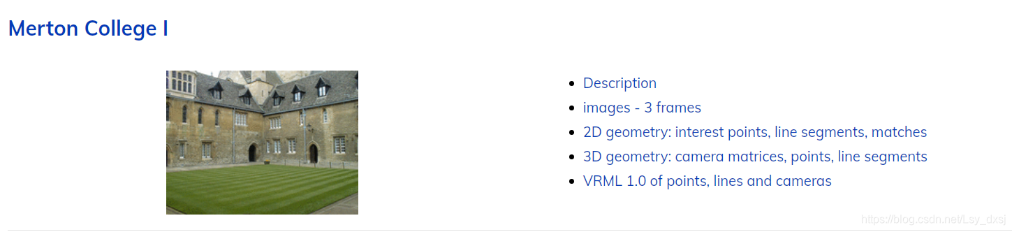
5.1.1 一个简单的数据集

数据集下载地址：https://www.robots.ox.ac.uk/~vgg/data/mview/
在这里插入图片描述
下载相应文件并解压在当前目录。

使用下面的代码，可加载Merton College I 的数据：

# -*- coding: utf-8 -*-
import camera#载入一些图像
im1 = array(Image.open('001.jpg'))
im2 = array(Image.open('002.jpg'))#载入每个视图的二维点到列表中
points2D = [loadtxt('00'+str(i+1)+'.corners').T for i in range(3)]
#载入三维点
points3D = loadtxt('p3d').T
#载入对应
corr = genfromtxt('nview-corners',dtype='int',missing_values='*')
#载入照相机矩阵到Camera对象列表中
P = [camera.Camera(loadtxt('00'+str(i+1)+'.P')) for i in range(3)]

上面的程序会加载前两个图像（共三个）、三个视图中的所有图像特征点、对应不同视图图像点重建后的三维点以及照相机参数矩阵。

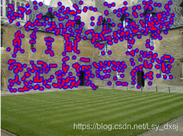
下面的代码可绘制出第一个视图以及该视图中的图像点。

# make 3D points homogeneous and project
X = vstack((points3D,ones(points3D.shape[1])))
x = P[0].project(X)# plotting the points in view 1
figure()
imshow(im1)
plot(points2D[0][0],points2D[0][1],'*')
axis('off')figure()
imshow(im1)
plot(x[0],x[1],'r.')
axis('off')
show()

运行结果如下：
在这里插入图片描述

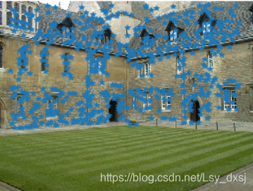
第二幅图比第一幅图多一些点，这些多出的点是从视图2和视图3重建出来的，而不在视图1中。

5.1.2 用Matplotlib绘制三维数据

为了可视化三维重建结果，需要绘制出三维图像。
用Matplotlib中的mplot3d工具包可以方便地绘制出三维点、线、等轮廓线、表面以及其他基本图像组件，还可以通过图像窗口控件实现三维旋转和缩放。

用以下代码实现三维绘图：

# -*- coding: utf-8 -*-
from mpl_toolkits.mplot3d import axes3dfig = figure()
ax = fig.gca(projection="3d")
ax.plot(points3D[0],points3D[1],points3D[2],'k.')#生成三维采样点
X,Y,Z = axes3d.get_test_data(0.25)#在三维中绘制点
ax.plot(X.flatten(),Y.flatten(),Z.flatten(),'o')
show()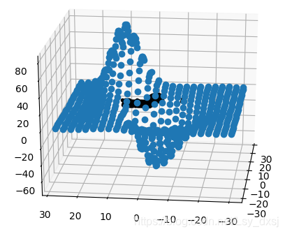

在这里插入图片描述

接下来，我们可以画出Merton样本数据来观察三维点的效果：

from mpl_toolkits.mplot3d import axes3dfig = figure()
ax = fig.gca(projection="3d")
ax.plot(points3D[0],points3D[1],points3D[2],'k.')
show()

运行结果如下：
在这里插入图片描述
在jupyter上运行如上图所示，图像不可旋转，接下来用sublime，运行结果可以对三维图像进行旋转，得到的运行结果如下：
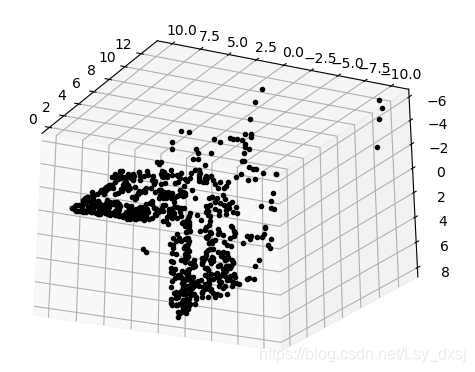（上面和侧边观测的视图）

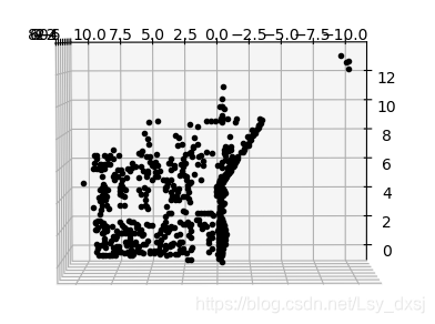
在这里插入图片描述（俯视的视图，展示了建筑墙体和屋顶上的点）
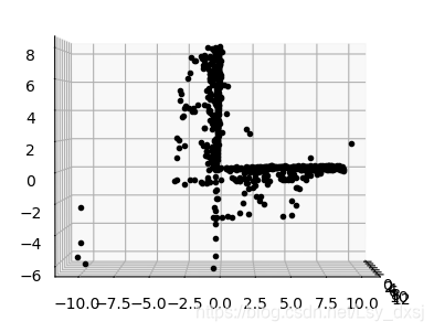
（侧视图，展示了一面墙的轮廓，以及另一面墙上点的主视图）

5.1.3 计算F：八点法

“八点法”指通过8个对应点计算基础矩阵F
对外极约束条件进行分析：
$x_2^TFx_1=0$
$\begin{bmatrix}x_{2}^{i}& y_{2}^{i}& w_{2}^{i}\end{bmatrix} \begin{bmatrix} F_{11} & F_{12} &F_{13}\\F_{21} & F_{22} & F_{23}\\ F_{31} & F_{32} & F_{33} \\ \end{bmatrix}\begin{bmatrix}x_{1}^{i}\\ y_{1}^{i}\\ w_{1}^{i}\end{bmatrix}=0$
（令 w = 1来归一化点）
$\left[\begin{array}{ccccc} x_{2}^{1} x_{1}^{1} & x_{2}^{1} y_{1}^{1} & x_{2}^{1} w_{1}^{1} & \cdots & w_{2}^{1} w_{1}^{1} \\ x_{2}^{2} x_{1}^{2} & x_{2}^{2} y_{1}^{2} & x_{2}^{2} w_{1}^{2} & \cdots & w_{2}^{2} w_{1}^{2} \\ \vdots & \vdots & \vdots & \ddots & \vdots \\ x_{2}^{n} x_{1}^{n} & x_{2}^{n} y_{1}^{n} & x_{2}^{n} w_{1}^{n} & \cdots & w_{2}^{n} w_{1}^{n} \end{array}\right]\left[\begin{array}{c} F_{11} \\ F_{12} \\ F_{13} \\ \vdots \\ F_{33} \end{array}\right]=A f=0$
其中， $\mathbf{x}_{1}^{i}=\left[x_{1}^{i}, y_{1}^{i}, w_{1}^{i}\right]$ 和 $\mathbf{x}_{2}^{i}=\left[x_{2}^{i}, y_{2}^{i}, w_{2}^{i}\right]$ 是一对图像点，共有n对对应点。因为基础矩阵中有9个元素，而尺度是任意的，因此需要8个方程。

以下是八点法中最小化 $\lVert$ $A f$ $\lVert$ 的函数：

def compute_fundamental(x1,x2):

但上面的的函数没有对图像坐标进行归一化，可能会带来数值问题。

5.1.4 外极点和外极线

外极点指满足式 $Fe_1=0$ 的点，可通过计算F的零空间来得到。
从F中计算右极点的函数：

def compute_epipole(F):

左极点的获得方法类似上面的函数，只需使用F的转置即可。

在两幅图中，用不同的颜色将点和对应的外极线对应起来。

# -*- coding: utf-8 -*-
from pylab import *
from mpl_toolkits.mplot3d import axes3d
import sfm#在前两个视图中点的索引
ndx = (corr[:,0]>=0) & (corr[:,1]>=0)#获得坐标，并将其用齐次坐标表示
x1 = points2D[0][:,corr[ndx,0]]
x1 = vstack((x1,ones(x1.shape[1])))
x2 = points2D[1][:,corr[ndx,1]]
x2 = vstack((x2,ones(x2.shape[1])))#计算F
F = sfm.compute_fundamental(x1,x2)#计算极点
e = sfm.compute_epipole(F)#绘制图像
figure()
imshow(im1)#分别绘制每条线，这样会绘制出很漂亮的颜色
for i in range(5):sfm.plot_epipolar_line(im1,F,x2[:,i],e,False)
axis('off')figure()
imshow(im2)#分别绘制每个点，这样绘制出和线同样的颜色
for i in range(5):plot(x2[0,i],x2[1,i],'o')
axis('off')
show()

运行结果为：
在这里插入图片描述

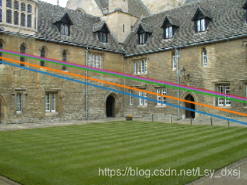
上面的代码首先选择了两幅图像的对应点，然后把它们转换成齐次坐标。由于缺失的数据在对应列表 corr 中为 -1，所以程序中有可能选取这些点。因此，上面的程序通过数组操作符 & 只选取了索引大于等于 0 的点。

对应点的选取方法有：

文本文件中读取
第二章，提取图像特征，再进行匹配

5.2 照相机和三维结构的计算

本节主要介绍计算照相机参数和三维结构的工具

5.2.1 三角剖分

给定照相机参数模型，图像点可以通过三角剖分来恢复这些点的三维位置对于两个照相机 P₁ 和 P₂ 的视图，三维实物点 X 的投影点为 x₁ 和 x₂（这里用齐次坐标表示），照相机方程定义了下列关系：
$\left[\begin{array}{ccc} P_{1} & -\mathbf{x}_{1} & 0 \\ P_{2} & 0 & -\mathbf{x}_{2} \end{array}\right]\left[\begin{array}{l} \mathbf{X} \\ \lambda_{1} \\ \lambda_{2} \end{array}\right]=0$
由于图像噪声、照相机参数误差和其他系统误差，上面的方程可能没有精确解。我
们可以通过 SVD 算法来得到三维点的最小二乘估值。

利用下面的代码来实现 Merton1 数据集上的三角剖分:


# -*- coding: utf-8 -*-
from pylab import *
from mpl_toolkits.mplot3d import axes3d
import sfm
# 在前两个视图中点的索引
ndx = (corr[:,0]>=0) & (corr[:,1]>=0)
# 获得坐标，并将其用齐次坐标表示
x1 = points2D[0][:,corr[ndx,0]]
x1 = vstack((x1,ones(x1.shape[1])))
x2 = points2D[1][:,corr[ndx,1]]
x2 = vstack((x2,ones(x2.shape[1])))
Xtrue = points3D[:,ndx]
Xtrue = vstack( (Xtrue,ones(Xtrue.shape[1])) )
# 检查前三个点
Xest = sfm.triangulate(x1,x2,P[0].P,P[1].P)
print (Xest[:,:3])
print (Xtrue[:,:3])
# 绘制图像
fig = figure()
ax = fig.gca(projection='3d')
ax.plot(Xest[0],Xest[1],Xest[2],'ko')
ax.plot(Xtrue[0],Xtrue[1],Xtrue[2],'r.')
axis('equal')
#axis('off')
show()

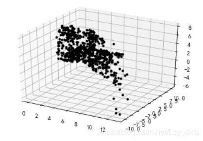
上面的代码利用前两个视图的信息来对图像点进行三角剖分，然后把前三个图像点的齐次坐标输出到控制台，然后绘制出恢复的最接近三维图像点。输出到控制台的信息如下：
在这里插入图片描述
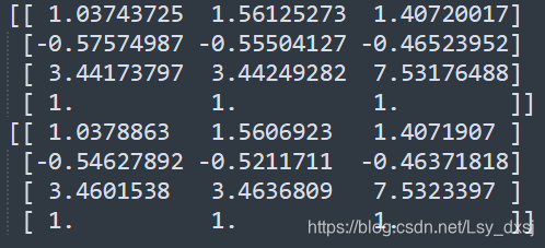
算法估计出的三维图像点和实际图像点很接近，如下图所示，估计点（黑色点）和实际点（红色点）可以很好的匹配。

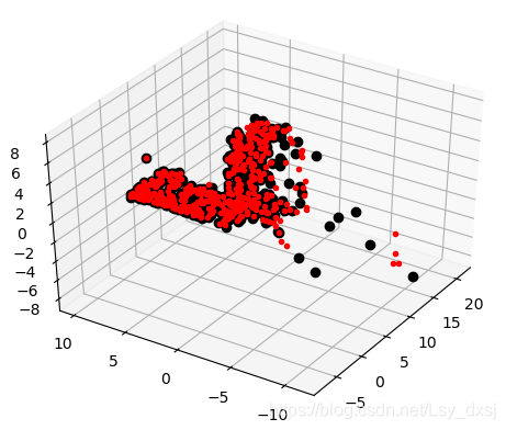
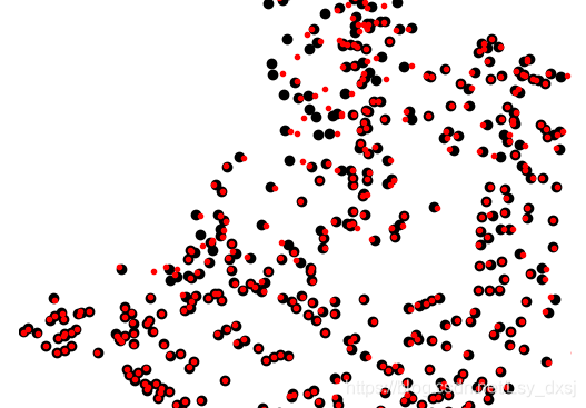
为了方便观察，选取了某一角度的图像点进行放大，如下图所示

在这里插入图片描述

5.2.2 由三维点计算照相机矩阵

也称为“照相机反切法”

已知一些三维点及其图像投影则可使用直接线性变换来计算照相机矩阵P，利用该方法恢复照相机矩阵同样是一个最小二乘问题。，可以利用SVD分解估计出照相机矩阵。

下面在我们的样本数据集上测试算法的性能，选出第一个视图中的一些可见点，将它们转换成齐次坐标表示，然后估计照相机矩阵。

# -*- coding: utf-8 -*-import camera
import numpy as np
from PIL import Image
from pylab import *im1 = array(Image.open('001.jpg'))
im2 = array(Image.open('002.jpg'))points2D = [loadtxt('00'+str(i+1)+'.corners').T for i in range(3)]
points3D = loadtxt('p3d').T
corr = genfromtxt('nview-corners',dtype='int',missing_values='*')
P = [camera.Camera(loadtxt('00'+str(i+1)+'.P')) for i in range(3)]corr = corr[:,0] # 视图 1
ndx3D = where(corr>=0)[0] # 丢失的数值为 -1
ndx2D = corr[ndx3D]
# 选取可见点，并用齐次坐标表示
x = points2D[0][:,ndx2D] # 视图 1
x = vstack( (x,ones(x.shape[1])) )
X = points3D[:,ndx3D]
X = vstack( (X,ones(X.shape[1])) )
# 估计 P
Pest = camera.Camera(sfm.compute_P(x,X))
# 比较！
print (Pest.P/Pest.P[2,3])
print (P[0].P/P[0].P[2, 3])
xest = Pest.project(X)
# 绘制图像
figure()
imshow(im1)
plot(x[0],x[1],'bo')
plot(xest[0],xest[1],'r.')
axis('off')
show()

归一化格式如下（可检查照相机矩阵的正确性）：
在这里插入图片描述
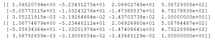
上面是估计出的照相机矩阵，下面是数据集的创造者计算出的照相机矩阵，他们的元素几乎完全相同。

使用估计出的照相机矩阵投影这些三维点，绘制出最后的投影结果，如下图所示（真实点用圆圈表示，估计出的投影点用点表示）：
在这里插入图片描述

5.2.3 由基础矩阵计算照相机矩阵

在两个视图场景中，照相机矩阵可以由基础矩阵恢复出来。研究分为两类：未标定的情况和已标定的情况。

未标定——投影重建
在没有任何照相机内参数知识的情况下，照相机矩阵只能通过射影变换恢复出来，即如果利用照相机的信息来重建三维点，那么该重建只有射影变换计算出来。
因此在无标定的情况下，第二个照相机矩阵可以使用一个（3×3）的射影变换得出。
$P_2=[S_eF|e]$
e是左极点，满足 $e^TF=0$
P.S. 使用该矩阵做出的三角形剖分很有可能会发生畸变，如倾斜的重建

def compute_P_from_fundamental(F):

def skew(a):

已标定——度量重建
在已标定的情况下，重建会保持欧氏空间中的一些度量特性（除了全局的尺度参数），在新的坐标系下，照相机方程变为：
$x_k=K^{-1}K[R|t]X=[R|t]X$
P.S. 在标定归一化的坐标系下，基础矩阵称为本质矩阵。为了区别为标定后的情况，以及归一化了的图像坐标，我们通常将其记为E，而非F

def compute_P_from_essential(E):

5.3 多视图重建

即从多幅图中计算出真实的三维重建

步骤：
(1) 检测特征点，然后在两幅图像间匹配；
(2) 由匹配计算基础矩阵；
(3) 由基础矩阵计算照相机矩阵；
(4) 三角剖分这些三维点。

5.3.1 稳健估计基础矩阵

类似于3.3节，使用的是RANSAC方法。

class RansacModel(object):

八点算法在平面场景中会失效，所以如果场景点都位于二维平面上，就不能使用该算法。

def compute_fundamental_normalized(x1,x2):

与单应性矩阵估计相比，增加了默认的最大迭代次数，改变了匹配的阈值。

def F_from_ransac(x1,x2,model,maxiter=5000,match_theshold=1e-6):

5.3.2 三维重建示例

先算出标定矩阵K：

def my_calibration(sz):row, col = szfx = 2555 * col / 2592fy = 2586 * row / 1936K = diag([fx, fy, 1])K[0, 2] = 0.5 * colK[1, 2] = 0.5 * rowreturn K

再进行三维重建：

# -*- coding: utf-8 -*-
from PIL import Image
from numpy import *
from pylab import *
import numpy as np
import camera
import homography
import sfm
import sift# 标定矩阵
# K = array([[2394,0,932],[0,2398,628],[0,0,1]])
K = my_calibration((1024,768))
# 载入图像，并计算特征im1 = array(Image.open('001.jpg'))
sift.process_image('001.jpg', '001.sift')
l1, d1 = sift.read_features_from_file('001.sift')im2 = array(Image.open('002.jpg'))
sift.process_image('002.jpg', '002.sift')
l2, d2 = sift.read_features_from_file('002.sift')# 匹配特征
matches = sift.match_twosided(d1,d2)
ndx = matches.nonzero()[0]# 使用齐次坐标表示，并使用 inv(K) 归一化
x1 = homography.make_homog(l1[ndx,:2].T)
ndx2 = [int(matches[i]) for i in ndx]
x2 = homography.make_homog(l2[ndx2,:2].T)
x1n = dot(inv(K),x1)
x2n = dot(inv(K),x2)# 使用 RANSAC 方法估计 E
model = sfm.RansacModel()
E,inliers = sfm.F_from_ransac(x1n,x2n,model)
# 计算照相机矩阵（P2 是 4 个解的列表）
P1 = array([[1,0,0,0],[0,1,0,0],[0,0,1,0]])
P2 = sfm.compute_P_from_essential(E)# 选取点在照相机前的解
ind = 0
maxres = 0
for i in range(4):# 三角剖分正确点，并计算每个照相机的深度X = sfm.triangulate(x1n[:,inliers],x2n[:,inliers],P1,P2[i])d1 = dot(P1,X)[2]d2 = dot(P2[i],X)[2]if sum(d1>0)+sum(d2>0) > maxres:maxres = sum(d1>0)+sum(d2>0)ind = iinfront = (d1>0) & (d2>0)# 三角剖分正确点，并移除不在所有照相机前面的点X = sfm.triangulate(x1n[:,inliers],x2n[:,inliers],P1,P2[ind])X = X[:,infront]# # 绘制三维图像
# from mpl_toolkits.mplot3d import axes3d
# fig = figure()
# ax = fig.gca(projection='3d')
# ax.plot(-X[0], X[1], X[2], 'k.')
# axis('off')# 绘制 X 的投影 import camera
# 绘制三维点
cam1 = camera.Camera(P1)
cam2 = camera.Camera(P2[ind])
x1p = cam1.project(X)
x2p = cam2.project(X)# 反 K 归一化
x1p = dot(K, x1p)
x2p = dot(K, x2p)
figure()
subplot(121)
imshow(im1)
gray()
plot(x1p[0], x1p[1], 'o')
plot(x1[0], x1[1], 'r.')
axis('off')subplot(122)
imshow(im2)
gray()
plot(x2p[0], x2p[1], 'o')
plot(x2[0], x2[1], 'r.')
axis('off')figure()
subplot(121)
plot(x1[0], x1[1], 'r.')
axis('off')subplot(122)
plot(x2[0], x2[1], 'r.')
axis('off')show()

运行结果如下：
在这里插入图片描述

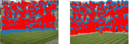
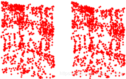
可以看到，二次投影后的点和原始特征位置不完全匹配，但是相当接近。

sfm.py

from pylab import *
from numpy import *
from scipy import linalgdef compute_P(x,X):"""    Compute camera matrix from pairs of2D-3D correspondences (in homog. coordinates). """n = x.shape[1]if X.shape[1] != n:raise ValueError("Number of points don't match.")# create matrix for DLT solutionM = zeros((3*n,12+n))for i in range(n):M[3*i,0:4] = X[:,i]M[3*i+1,4:8] = X[:,i]M[3*i+2,8:12] = X[:,i]M[3*i:3*i+3,i+12] = -x[:,i]U,S,V = linalg.svd(M)return V[-1,:12].reshape((3,4))def triangulate_point(x1,x2,P1,P2):""" Point pair triangulation from least squares solution. """M = zeros((6,6))M[:3,:4] = P1M[3:,:4] = P2M[:3,4] = -x1M[3:,5] = -x2U,S,V = linalg.svd(M)X = V[-1,:4]return X / X[3]def triangulate(x1,x2,P1,P2):"""    Two-view triangulation of points in x1,x2 (3*n homog. coordinates). """n = x1.shape[1]if x2.shape[1] != n:raise ValueError("Number of points don't match.")X = [ triangulate_point(x1[:,i],x2[:,i],P1,P2) for i in range(n)]return array(X).Tdef compute_fundamental(x1,x2):"""    Computes the fundamental matrix from corresponding points (x1,x2 3*n arrays) using the 8 point algorithm.Each row in the A matrix below is constructed as[x'*x, x'*y, x', y'*x, y'*y, y', x, y, 1] """n = x1.shape[1]if x2.shape[1] != n:raise ValueError("Number of points don't match.")# build matrix for equationsA = zeros((n,9))for i in range(n):A[i] = [x1[0,i]*x2[0,i], x1[0,i]*x2[1,i], x1[0,i]*x2[2,i],x1[1,i]*x2[0,i], x1[1,i]*x2[1,i], x1[1,i]*x2[2,i],x1[2,i]*x2[0,i], x1[2,i]*x2[1,i], x1[2,i]*x2[2,i] ]# compute linear least square solutionU,S,V = linalg.svd(A)F = V[-1].reshape(3,3)# constrain F# make rank 2 by zeroing out last singular valueU,S,V = linalg.svd(F)S[2] = 0F = dot(U,dot(diag(S),V))return F/F[2,2]def compute_epipole(F):""" Computes the (right) epipole from a fundamental matrix F. (Use with F.T for left epipole.) """# return null space of F (Fx=0)U,S,V = linalg.svd(F)e = V[-1]return e/e[2]def plot_epipolar_line(im,F,x,epipole=None,show_epipole=True):""" Plot the epipole and epipolar line F*x=0in an image. F is the fundamental matrix and x a point in the other image."""m,n = im.shape[:2]line = dot(F,x)# epipolar line parameter and valuest = linspace(0,n,100)lt = array([(line[2]+line[0]*tt)/(-line[1]) for tt in t])# take only line points inside the imagendx = (lt>=0) & (lt<m) plot(t[ndx],lt[ndx],linewidth=2)if show_epipole:if epipole is None:epipole = compute_epipole(F)plot(epipole[0]/epipole[2],epipole[1]/epipole[2],'r*')def skew(a):""" Skew matrix A such that a x v = Av for any v. """return array([[0,-a[2],a[1]],[a[2],0,-a[0]],[-a[1],a[0],0]])def compute_P_from_fundamental(F):"""    Computes the second camera matrix (assuming P1 = [I 0]) from a fundamental matrix. """e = compute_epipole(F.T) # left epipoleTe = skew(e)return vstack((dot(Te,F.T).T,e)).Tdef compute_P_from_essential(E):"""    Computes the second camera matrix (assuming P1 = [I 0]) from an essential matrix. Output is a list of four possible camera matrices. """# make sure E is rank 2U,S,V = svd(E)if det(dot(U,V))<0:V = -VE = dot(U,dot(diag([1,1,0]),V))    # create matrices (Hartley p 258)Z = skew([0,0,-1])W = array([[0,-1,0],[1,0,0],[0,0,1]])# return all four solutionsP2 = [vstack((dot(U,dot(W,V)).T,U[:,2])).T,vstack((dot(U,dot(W,V)).T,-U[:,2])).T,vstack((dot(U,dot(W.T,V)).T,U[:,2])).T,vstack((dot(U,dot(W.T,V)).T,-U[:,2])).T]return P2def compute_fundamental_normalized(x1,x2):"""    Computes the fundamental matrix from corresponding points (x1,x2 3*n arrays) using the normalized 8 point algorithm. """n = x1.shape[1]if x2.shape[1] != n:raise ValueError("Number of points don't match.")# normalize image coordinatesx1 = x1 / x1[2]mean_1 = mean(x1[:2],axis=1)S1 = sqrt(2) / std(x1[:2])T1 = array([[S1,0,-S1*mean_1[0]],[0,S1,-S1*mean_1[1]],[0,0,1]])x1 = dot(T1,x1)x2 = x2 / x2[2]mean_2 = mean(x2[:2],axis=1)S2 = sqrt(2) / std(x2[:2])T2 = array([[S2,0,-S2*mean_2[0]],[0,S2,-S2*mean_2[1]],[0,0,1]])x2 = dot(T2,x2)# compute F with the normalized coordinatesF = compute_fundamental(x1,x2)# reverse normalizationF = dot(T1.T,dot(F,T2))return F/F[2,2]class RansacModel(object):""" Class for fundmental matrix fit with ransac.py fromhttp://www.scipy.org/Cookbook/RANSAC"""def __init__(self,debug=False):self.debug = debugdef fit(self,data):""" Estimate fundamental matrix using eight selected correspondences. """# transpose and split data into the two point setsdata = data.Tx1 = data[:3,:8]x2 = data[3:,:8]# estimate fundamental matrix and returnF = compute_fundamental_normalized(x1,x2)return Fdef get_error(self,data,F):""" Compute x^T F x for all correspondences, return error for each transformed point. """# transpose and split data into the two pointdata = data.Tx1 = data[:3]x2 = data[3:]# Sampson distance as error measureFx1 = dot(F,x1)Fx2 = dot(F,x2)denom = Fx1[0]**2 + Fx1[1]**2 + Fx2[0]**2 + Fx2[1]**2err = ( diag(dot(x1.T,dot(F,x2))) )**2 / denom # return error per pointreturn errdef F_from_ransac(x1,x2,model,maxiter=5000,match_theshold=1e-6):""" Robust estimation of a fundamental matrix F from point correspondences using RANSAC (ransac.py fromhttp://www.scipy.org/Cookbook/RANSAC).input: x1,x2 (3*n arrays) points in hom. coordinates. """from PCV.tools import ransacdata = vstack((x1,x2))# compute F and return with inlier indexF,ransac_data = ransac.ransac(data.T,model,8,maxiter,match_theshold,20,return_all=True)return F, ransac_data['inliers']