电力负荷预测
- 电力分析与预测
- 一.导入数据
- 二.数据的预处理
- 三.基本描述性统计
- 四.构建特征,模型准备
- ①系统聚类法
- ②K-means聚类
- 五.构建特征,建立预测模型
- ①预测未来一天,各时段的电力负荷
- ②预测未来几天总体电力负荷
电力分析与预测
根据提供的客户的20天的分时段数据,进行分析:
要求1:根据数据对客户进行聚类分析;
要求2:根据数据对客户进行负荷预测。
一.导入数据
# 安装库专用# 通过如下命令设定镜像
options(repos = 'http://mirrors.ustc.edu.cn/CRAN/')
# 查看镜像是否修改
getOption('repos')
# 尝试下载R包
#若有需要,进行安装
#install.packages('forecast')
‘http://mirrors.ustc.edu.cn/CRAN/’
Installing package into 'C:/Users/天涯过客/Documents/R/win-library/4.0'
(as 'lib' is unspecified)also installing the dependencies 'fracdiff', 'urca'package 'fracdiff' successfully unpacked and MD5 sums checked
package 'urca' successfully unpacked and MD5 sums checked
package 'forecast' successfully unpacked and MD5 sums checkedThe downloaded binary packages are inC:\Users\天涯过客\AppData\Local\Temp\Rtmpop8xQR\downloaded_packages
#设置工作路径
setwd("D:/LengPY")
#导入数据
library(readxl)
data1_6<-read_excel("10.1-10.6日数据.xlsx",sheet=1)
data7_13<-read_excel("10.7-10.13日数据.xlsx",sheet=1)
data14_20<-read_excel("10.14-10.20日数据.xlsx",sheet=1)
head(data1_6,3)
| id | date | 00:00-00:15 | 00:15-00:30 | 00:30-00:45 | 00:45-01:00 | 01:00-01:15 | 01:15-01:30 | 01:30-01:45 | 01:45-02:00 | ... | 21:30-21:45 | 21:45-22:00 | 22:00-22:15 | 22:15-22:30 | 22:30-22:45 | 22:45-23:00 | 23:00-23:15 | 23:15-23:30 | 23:30-23:45 | 23:45-00:00 |
|---|---|---|---|---|---|---|---|---|---|---|---|---|---|---|---|---|---|---|---|---|
| <chr> | <chr> | <dbl> | <dbl> | <dbl> | <dbl> | <dbl> | <dbl> | <dbl> | <dbl> | ... | <dbl> | <dbl> | <dbl> | <dbl> | <dbl> | <dbl> | <dbl> | <dbl> | <dbl> | <dbl> |
| 客户4 | 2020-10-01 | 0.619 | 0.619 | 0.619 | 0.619 | 0.619 | 0.619 | 0.619 | 0.619 | ... | 0.581 | 0.581 | 0.581 | 0.581 | 0.581 | 0.581 | 0.619 | 0.619 | 0.619 | 0.619 |
| 客户5 | 2020-10-01 | 3.210 | 3.210 | 3.210 | 3.210 | 3.210 | 3.210 | 3.210 | 3.210 | ... | 3.210 | 3.210 | 3.210 | 3.210 | 3.210 | 3.210 | 3.210 | 3.210 | 3.210 | 3.210 |
| 客户8 | 2020-10-01 | 0.000 | 0.000 | 0.000 | 0.000 | 0.000 | 0.000 | 0.000 | 0.000 | ... | 0.000 | 0.000 | 0.000 | 0.000 | 0.000 | 0.000 | 0.000 | 0.000 | 0.000 | 0.000 |
二.数据的预处理
#head(data7_13,3)
#head(data14_20,3)
### 可发现维度一致,将其合并
data<-rbind(data1_6,data7_13,data14_20)
head(data)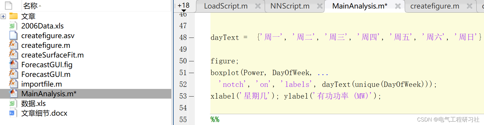
str(data)#查看数据类型| id | date | 00:00-00:15 | 00:15-00:30 | 00:30-00:45 | 00:45-01:00 | 01:00-01:15 | 01:15-01:30 | 01:30-01:45 | 01:45-02:00 | ... | 21:30-21:45 | 21:45-22:00 | 22:00-22:15 | 22:15-22:30 | 22:30-22:45 | 22:45-23:00 | 23:00-23:15 | 23:15-23:30 | 23:30-23:45 | 23:45-00:00 |
|---|---|---|---|---|---|---|---|---|---|---|---|---|---|---|---|---|---|---|---|---|
| <chr> | <chr> | <dbl> | <dbl> | <dbl> | <dbl> | <dbl> | <dbl> | <dbl> | <dbl> | ... | <dbl> | <dbl> | <dbl> | <dbl> | <dbl> | <dbl> | <dbl> | <dbl> | <dbl> | <dbl> |
| 客户4 | 2020-10-01 | 0.619 | 0.619 | 0.619 | 0.619 | 0.619 | 0.619 | 0.619 | 0.619 | ... | 0.581 | 0.581 | 0.581 | 0.581 | 0.581 | 0.581 | 0.619 | 0.619 | 0.619 | 0.619 |
| 客户5 | 2020-10-01 | 3.210 | 3.210 | 3.210 | 3.210 | 3.210 | 3.210 | 3.210 | 3.210 | ... | 3.210 | 3.210 | 3.210 | 3.210 | 3.210 | 3.210 | 3.210 | 3.210 | 3.210 | 3.210 |
| 客户8 | 2020-10-01 | 0.000 | 0.000 | 0.000 | 0.000 | 0.000 | 0.000 | 0.000 | 0.000 | ... | 0.000 | 0.000 | 0.000 | 0.000 | 0.000 | 0.000 | 0.000 | 0.000 | 0.000 | 0.000 |
| 客户7 | 2020-10-01 | 0.625 | 0.625 | 0.625 | 0.625 | 0.625 | 0.625 | 0.625 | 0.625 | ... | 0.635 | 0.635 | 0.635 | 0.635 | 0.635 | 0.635 | 0.625 | 0.625 | 0.625 | 0.625 |
| 客户89 | 2020-10-01 | 22.278 | 22.278 | 22.278 | 22.278 | 22.278 | 22.278 | 22.278 | 22.278 | ... | 14.470 | 14.470 | 14.470 | 14.470 | 14.470 | 14.470 | 22.278 | 22.278 | 22.278 | 22.278 |
| 客户160 | 2020-10-01 | 65.200 | 48.480 | 65.840 | 62.560 | 49.120 | 64.560 | 62.560 | 65.840 | ... | 84.560 | 85.920 | 85.920 | 83.920 | 84.560 | 67.200 | 98.000 | 83.920 | 84.560 | 98.640 |
tibble [3,900 x 98] (S3: tbl_df/tbl/data.frame)$ id : chr [1:3900] "客户4" "客户5" "客户8" "客户7" ...$ date : chr [1:3900] "2020-10-01" "2020-10-01" "2020-10-01" "2020-10-01" ...$ 00:00-00:15: num [1:3900] 0.619 3.21 0 0.625 22.278 ...$ 00:15-00:30: num [1:3900] 0.619 3.21 0 0.625 22.278 ...$ 00:30-00:45: num [1:3900] 0.619 3.21 0 0.625 22.278 ...$ 00:45-01:00: num [1:3900] 0.619 3.21 0 0.625 22.278 ...$ 01:00-01:15: num [1:3900] 0.619 3.21 0 0.625 22.278 ...$ 01:15-01:30: num [1:3900] 0.619 3.21 0 0.625 22.278 ...$ 01:30-01:45: num [1:3900] 0.619 3.21 0 0.625 22.278 ...$ 01:45-02:00: num [1:3900] 0.619 3.21 0 0.625 22.278 ...$ 02:00-02:15: num [1:3900] 0.619 3.21 0 0.625 22.278 ...$ 02:15-02:30: num [1:3900] 0.619 3.21 0 0.625 22.278 ...$ 02:30-02:45: num [1:3900] 0.619 3.21 0 0.625 22.278 ...$ 02:45-03:00: num [1:3900] 0.619 3.21 0 0.625 22.278 ...$ 03:00-03:15: num [1:3900] 0.619 3.21 0 0.625 22.278 ...$ 03:15-03:30: num [1:3900] 0.619 3.21 0 0.625 22.278 ...$ 03:30-03:45: num [1:3900] 0.619 3.21 0 0.625 22.278 ...$ 03:45-04:00: num [1:3900] 0.619 3.21 0 0.625 22.278 ...$ 04:00-04:15: num [1:3900] 0.619 3.21 0 0.625 22.278 ...$ 04:15-04:30: num [1:3900] 0.619 3.21 0 0.625 22.278 ...$ 04:30-04:45: num [1:3900] 0.619 3.21 0 0.625 22.278 ...$ 04:45-05:00: num [1:3900] 0.619 3.21 0 0.625 22.278 ...$ 05:00-05:15: num [1:3900] 0.619 3.21 0 0.625 22.278 ...$ 05:15-05:30: num [1:3900] 0.619 3.21 0 0.625 22.278 ...$ 05:30-05:45: num [1:3900] 0.619 3.21 0 0.625 22.278 ...$ 05:45-06:00: num [1:3900] 0.619 3.21 0 0.625 22.278 ...$ 06:00-06:15: num [1:3900] 0.619 3.21 0 0.625 22.278 ...$ 06:15-06:30: num [1:3900] 0.619 3.21 0 0.625 22.278 ...$ 06:30-06:45: num [1:3900] 0.619 3.21 0 0.625 22.278 ...$ 06:45-07:00: num [1:3900] 0.619 3.21 0 0.625 22.278 ...$ 07:00-07:15: num [1:3900] 0.581 3.21 0 0.635 14.47 ...$ 07:15-07:30: num [1:3900] 0.581 3.21 0 0.635 14.47 ...$ 07:30-07:45: num [1:3900] 0.581 3.21 0 0.635 14.47 ...$ 07:45-08:00: num [1:3900] 0.581 3.21 0 0.635 14.47 ...$ 08:00-08:15: num [1:3900] 0.581 3.21 0 0.635 14.47 ...$ 08:15-08:30: num [1:3900] 0.581 3.21 0 0.635 14.47 ...$ 08:30-08:45: num [1:3900] 0.581 3.21 0 0.635 14.47 ...$ 08:45-09:00: num [1:3900] 0.581 3.21 0 0.635 14.47 ...$ 09:00-09:15: num [1:3900] 0.581 3.21 0 0.635 14.47 ...$ 09:15-09:30: num [1:3900] 0.581 3.21 0 0.635 14.47 ...$ 09:30-09:45: num [1:3900] 0.581 3.21 0 0.635 14.47 ...$ 09:45-10:00: num [1:3900] 0.581 3.21 0 0.635 14.47 ...$ 10:00-10:15: num [1:3900] 0.581 3.21 0 0.635 14.47 ...$ 10:15-10:30: num [1:3900] 0.581 3.21 0 0.635 14.47 ...$ 10:30-10:45: num [1:3900] 0.581 3.21 0 0.635 14.47 ...$ 10:45-11:00: num [1:3900] 0.581 3.21 0 0.635 14.47 ...$ 11:00-11:15: num [1:3900] 0.608 3.611 0 0.624 9.262 ...$ 11:15-11:30: num [1:3900] 0.608 3.611 0 0.624 9.262 ...$ 11:30-11:45: num [1:3900] 0.608 3.611 0 0.624 9.262 ...$ 11:45-12:00: num [1:3900] 0.608 3.611 0 0.624 9.262 ...$ 12:00-12:15: num [1:3900] 0.608 3.611 0 0.624 9.262 ...$ 12:15-12:30: num [1:3900] 0.608 3.611 0 0.624 9.262 ...$ 12:30-12:45: num [1:3900] 0.608 3.611 0 0.624 9.262 ...$ 12:45-13:00: num [1:3900] 0.608 3.611 0 0.624 9.262 ...$ 13:00-13:15: num [1:3900] 0.608 3.611 0 0.624 9.262 ...$ 13:15-13:30: num [1:3900] 0.608 3.611 0 0.624 9.262 ...$ 13:30-13:45: num [1:3900] 0.608 3.611 0 0.624 9.262 ...$ 13:45-14:00: num [1:3900] 0.608 3.611 0 0.624 9.262 ...$ 14:00-14:15: num [1:3900] 0.608 3.611 0 0.624 9.262 ...$ 14:15-14:30: num [1:3900] 0.608 3.611 0 0.624 9.262 ...$ 14:30-14:45: num [1:3900] 0.608 3.611 0 0.624 9.262 ...$ 14:45-15:00: num [1:3900] 0.608 3.611 0 0.624 9.262 ...$ 15:00-15:15: num [1:3900] 0.608 3.611 0 0.624 9.262 ...$ 15:15-15:30: num [1:3900] 0.608 3.611 0 0.624 9.262 ...$ 15:30-15:45: num [1:3900] 0.608 3.611 0 0.624 9.262 ...$ 15:45-16:00: num [1:3900] 0.608 3.611 0 0.624 9.262 ...$ 16:00-16:15: num [1:3900] 0.608 3.611 0 0.624 9.262 ...$ 16:15-16:30: num [1:3900] 0.608 3.611 0 0.624 9.262 ...$ 16:30-16:45: num [1:3900] 0.608 3.611 0 0.624 9.262 ...$ 16:45-17:00: num [1:3900] 0.608 3.611 0 0.624 9.262 ...$ 17:00-17:15: num [1:3900] 0.608 3.611 0 0.624 9.262 ...$ 17:15-17:30: num [1:3900] 0.608 3.611 0 0.624 9.262 ...$ 17:30-17:45: num [1:3900] 0.608 3.611 0 0.624 9.262 ...$ 17:45-18:00: num [1:3900] 0.608 3.611 0 0.624 9.262 ...$ 18:00-18:15: num [1:3900] 0.608 3.611 0 0.624 9.262 ...$ 18:15-18:30: num [1:3900] 0.608 3.611 0 0.624 9.262 ...$ 18:30-18:45: num [1:3900] 0.608 3.611 0 0.624 9.262 ...$ 18:45-19:00: num [1:3900] 0.608 3.611 0 0.624 9.262 ...$ 19:00-19:15: num [1:3900] 0.581 3.21 0 0.635 14.47 ...$ 19:15-19:30: num [1:3900] 0.581 3.21 0 0.635 14.47 ...$ 19:30-19:45: num [1:3900] 0.581 3.21 0 0.635 14.47 ...$ 19:45-20:00: num [1:3900] 0.581 3.21 0 0.635 14.47 ...$ 20:00-20:15: num [1:3900] 0.581 3.21 0 0.635 14.47 ...$ 20:15-20:30: num [1:3900] 0.581 3.21 0 0.635 14.47 ...$ 20:30-20:45: num [1:3900] 0.581 3.21 0 0.635 14.47 ...$ 20:45-21:00: num [1:3900] 0.581 3.21 0 0.635 14.47 ...$ 21:00-21:15: num [1:3900] 0.581 3.21 0 0.635 14.47 ...$ 21:15-21:30: num [1:3900] 0.581 3.21 0 0.635 14.47 ...$ 21:30-21:45: num [1:3900] 0.581 3.21 0 0.635 14.47 ...$ 21:45-22:00: num [1:3900] 0.581 3.21 0 0.635 14.47 ...$ 22:00-22:15: num [1:3900] 0.581 3.21 0 0.635 14.47 ...$ 22:15-22:30: num [1:3900] 0.581 3.21 0 0.635 14.47 ...$ 22:30-22:45: num [1:3900] 0.581 3.21 0 0.635 14.47 ...$ 22:45-23:00: num [1:3900] 0.581 3.21 0 0.635 14.47 ...$ 23:00-23:15: num [1:3900] 0.619 3.21 0 0.625 22.278 ...$ 23:15-23:30: num [1:3900] 0.619 3.21 0 0.625 22.278 ...$ 23:30-23:45: num [1:3900] 0.619 3.21 0 0.625 22.278 ...$ 23:45-00:00: num [1:3900] 0.619 3.21 0 0.625 22.278 ...
#检查是否有缺失值
## 可视化查看数据是否有缺失值
library(VIM)
aggr(data)
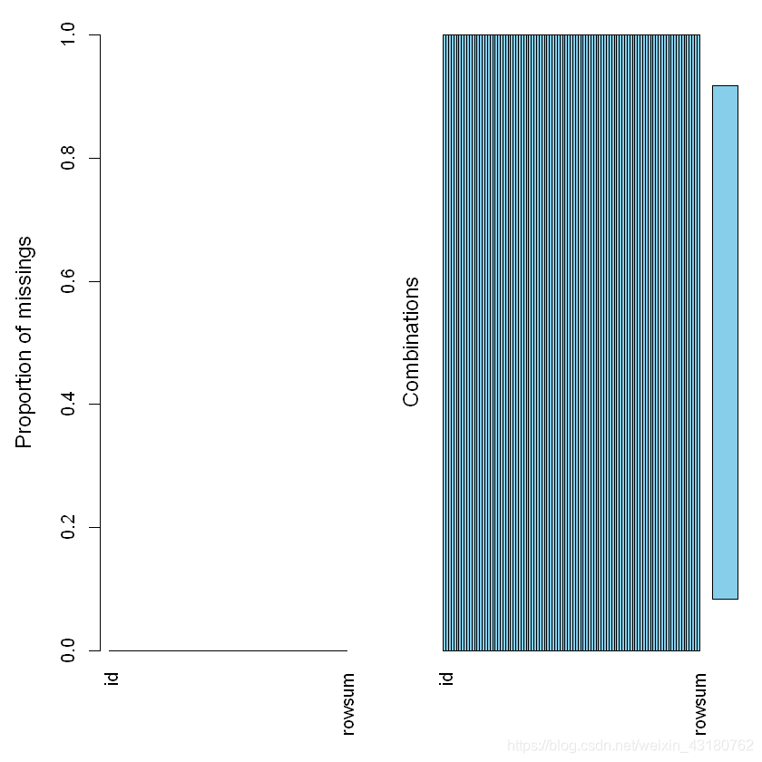
经检查,不存在缺失值,可直接进行分析。
# 按行计算总和
#library(dyplr)
library(tidyverse)
data<-data %>%mutate(rowsum = rowSums(.[3:98]))#添加一列,计算行和
三.基本描述性统计
#不同时间总负荷量对比
date_rowsum<-aggregate(x =data$rowsum, by= list(data$date), FUN =sum)
colnames(date_rowsum)<-c('date','sum')
date_rowsum
| date | sum |
|---|---|
| <chr> | <dbl> |
| 2020-10-01 | 93125.13 |
| 2020-10-02 | 89564.60 |
| 2020-10-03 | 89715.30 |
| 2020-10-04 | 91119.79 |
| 2020-10-05 | 95884.30 |
| 2020-10-06 | 95558.53 |
| 2020-10-07 | 97199.34 |
| 2020-10-08 | 97358.87 |
| 2020-10-09 | 91890.29 |
| 2020-10-10 | 94850.10 |
| 2020-10-11 | 95424.02 |
| 2020-10-12 | 100501.56 |
| 2020-10-13 | 100307.05 |
| 2020-10-14 | 101899.14 |
| 2020-10-15 | 105264.88 |
| 2020-10-16 | 105435.29 |
| 2020-10-17 | 100331.14 |
| 2020-10-18 | 103870.77 |
| 2020-10-19 | 99513.48 |
| 2020-10-20 | 95456.16 |
date_rowsum$date<-as.Date(date_rowsum$date)
plot(date_rowsum,type = "o", col = "red", xlab = "date", ylab = "sum",main = "date_sum")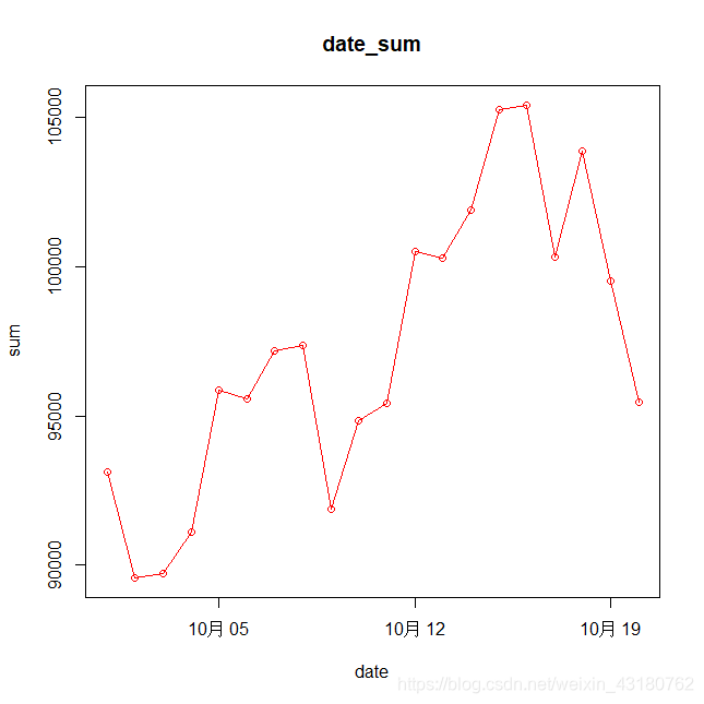
可发现在国庆节期间,电力负荷较低,可能与休假导致用电量下降有关,同时用电之间存在一定的周期性关系,推测是由于周末等因素导致周期性,可对此周期进行提取进一步分析。
#不同用户总负荷量对比
id_rowsum<-aggregate(x =data$rowsum, by= list(data$id), FUN =sum)
colnames(id_rowsum)<-c('id','sum')
head(id_rowsum)
| id | sum | |
|---|---|---|
| <chr> | <dbl> | |
| 1 | 客户10 | 880.640 |
| 2 | 客户100 | 1343.552 |
| 3 | 客户101 | 6545.280 |
| 4 | 客户102 | 5985.280 |
| 5 | 客户103 | 1501.560 |
| 6 | 客户104 | 94735.159 |
summary(id_rowsum)#计算用户数量
id sum Length:176 Min. : 0.0 Class :character 1st Qu.: 325.4 Mode :character Median : 892.7 Mean : 11047.0 3rd Qu.: 3533.8 Max. :164139.1
可知:样本有176名用户,其中平均总用电负荷11047,最高164139.1
hist(id_rowsum$sum, col = rgb(1,0,0,0.2))
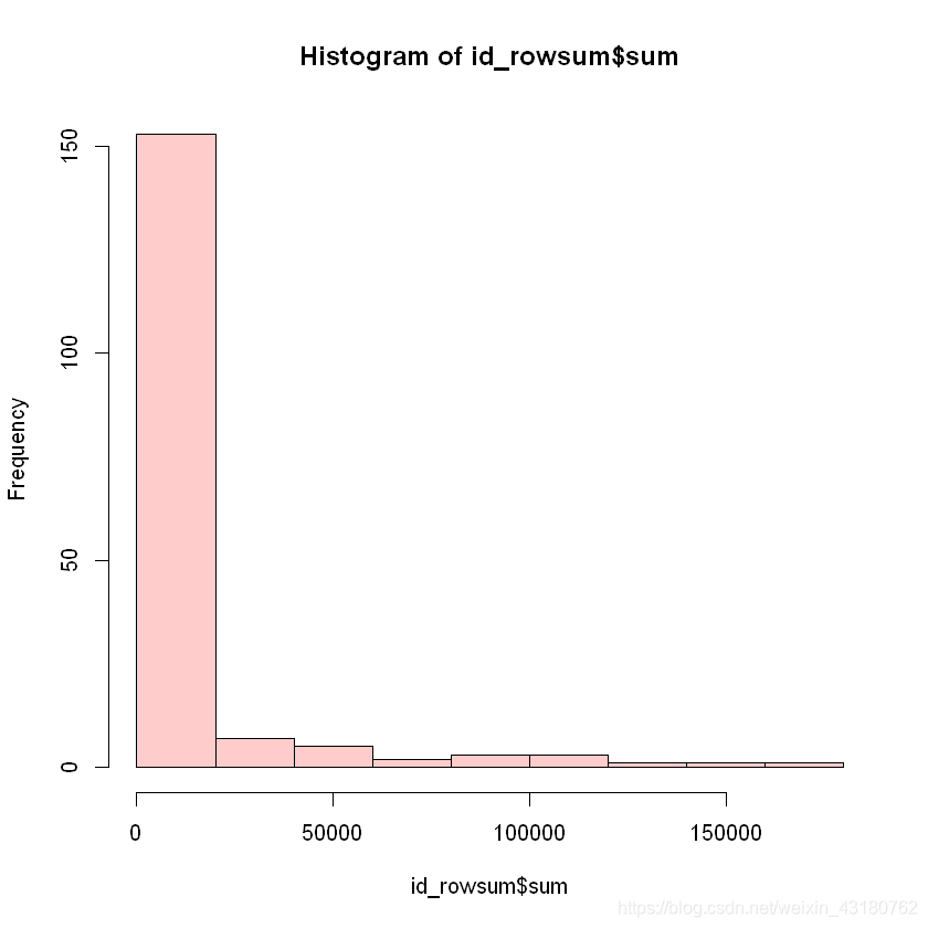
可发现,大部分客户消耗电力负荷在20000以内,数据分布呈现偏态分布,用电量高的用户占小部分。可根据电力负荷量使用量等对客户进行分类,实行不同的政策。
#不同用户不同时间负荷量对比
date_id_rowsum<-aggregate(x =data$rowsum, by= list(data$date,data$id), FUN =sum)
colnames(date_id_rowsum)<-c('date','id','sum')
head(date_id_rowsum)
| date | id | sum | |
|---|---|---|---|
| <chr> | <chr> | <dbl> | |
| 1 | 2020-10-01 | 客户10 | 44.032 |
| 2 | 2020-10-02 | 客户10 | 44.032 |
| 3 | 2020-10-03 | 客户10 | 44.032 |
| 4 | 2020-10-04 | 客户10 | 44.032 |
| 5 | 2020-10-05 | 客户10 | 44.032 |
| 6 | 2020-10-06 | 客户10 | 44.032 |
library(dplyr)
cdata<-as.tibble(data)
#转换格式,便于处理
#计算1-20日各时段总功率情况
hourdata<-data%>%select(-id)%>% summarise(across(contains(":"),sum,na.rm=TRUE))
hourdata<-as.data.frame(hourdata)
#进行转置
hourdatat<-t(hourdata)
hourdatat<-as.data.frame(hourdatat)
colnames(hourdatat)<-c('sum')
hourdatat$time<-rownames(hourdatat)
head(hourdatat)| sum | time | |
|---|---|---|
| <dbl> | <chr> | |
| 00:00-00:15 | 22090.48 | 00:00-00:15 |
| 00:15-00:30 | 22195.23 | 00:15-00:30 |
| 00:30-00:45 | 22047.53 | 00:30-00:45 |
| 00:45-01:00 | 22128.37 | 00:45-01:00 |
| 01:00-01:15 | 22152.18 | 01:00-01:15 |
| 01:15-01:30 | 22407.36 | 01:15-01:30 |
barplot(hourdatat$sum,names.arg=hourdatat$time,xlab="time",ylab="sum",col="blue",
main="sum_hour",border="red")
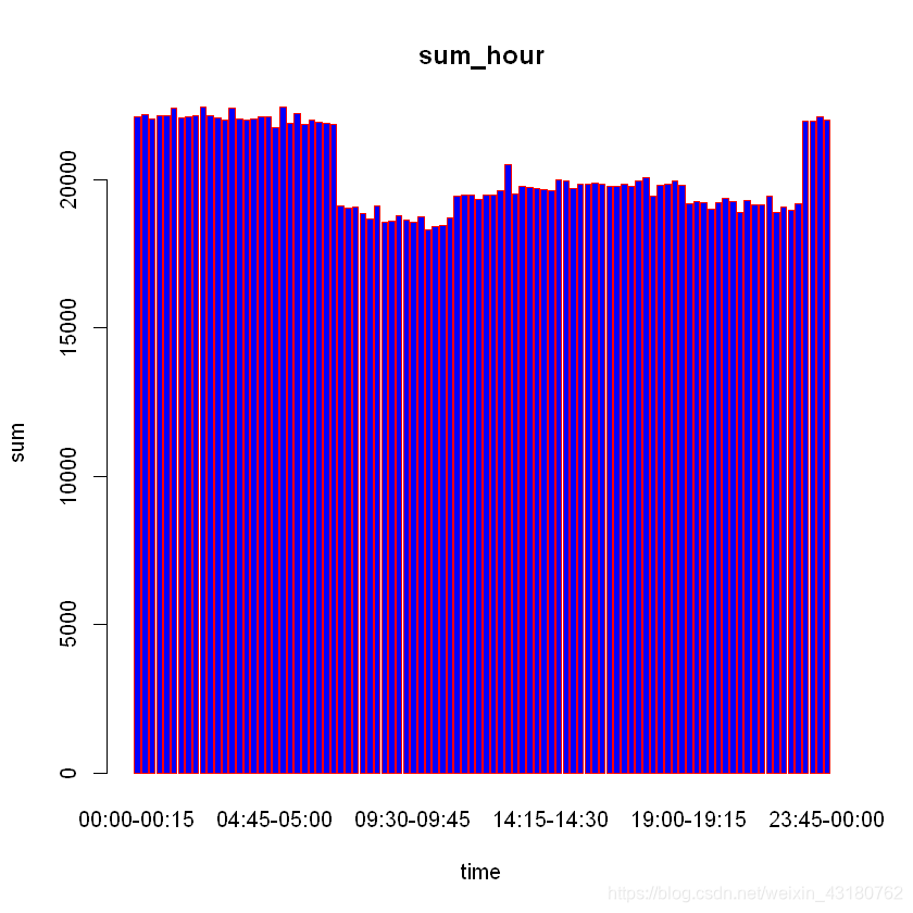
可根据时段统计,确定用电峰谷情况,可根据高峰期与低谷期进行区别定价和计划供电。本例由于样本点较少,故以上信息仅供参考。
四.构建特征,模型准备
#计算每用户各时段平均功率情况
hour_meanid<-cdata%>%select(-date)%>% group_by(id)%>%summarise(across(everything(),mean,na.rm=TRUE))
head(hour_meanid)
| id | 00:00-00:15 | 00:15-00:30 | 00:30-00:45 | 00:45-01:00 | 01:00-01:15 | 01:15-01:30 | 01:30-01:45 | 01:45-02:00 | 02:00-02:15 | ... | 21:45-22:00 | 22:00-22:15 | 22:15-22:30 | 22:30-22:45 | 22:45-23:00 | 23:00-23:15 | 23:15-23:30 | 23:30-23:45 | 23:45-00:00 | rowsum |
|---|---|---|---|---|---|---|---|---|---|---|---|---|---|---|---|---|---|---|---|---|
| <chr> | <dbl> | <dbl> | <dbl> | <dbl> | <dbl> | <dbl> | <dbl> | <dbl> | <dbl> | ... | <dbl> | <dbl> | <dbl> | <dbl> | <dbl> | <dbl> | <dbl> | <dbl> | <dbl> | <dbl> |
| 客户10 | 0.45400 | 0.45400 | 0.45400 | 0.45400 | 0.45400 | 0.45400 | 0.45400 | 0.45400 | 0.45400 | ... | 0.45400 | 0.45400 | 0.45400 | 0.45400 | 0.45400 | 0.45400 | 0.45400 | 0.45400 | 0.45400 | 44.0320 |
| 客户100 | 0.28375 | 0.28375 | 0.28375 | 0.28375 | 0.28375 | 0.28375 | 0.28375 | 0.28375 | 0.28375 | ... | 0.63815 | 0.63815 | 0.63815 | 0.63815 | 0.63815 | 0.28375 | 0.28375 | 0.28375 | 0.28375 | 67.1776 |
| 客户101 | 10.69600 | 10.36000 | 9.40800 | 10.41600 | 10.30400 | 10.64000 | 10.36000 | 10.36000 | 9.96800 | ... | 0.00000 | 0.00000 | 0.00000 | 0.00000 | 0.00000 | 10.30400 | 10.92000 | 10.02400 | 10.80800 | 327.2640 |
| 客户102 | 3.08600 | 3.08600 | 3.08600 | 3.08600 | 3.08600 | 3.08600 | 3.08600 | 3.08600 | 3.08600 | ... | 3.08600 | 3.08600 | 3.08600 | 3.08600 | 3.08600 | 3.08600 | 3.08600 | 3.08600 | 3.08600 | 299.2640 |
| 客户103 | 0.83400 | 0.76200 | 0.70200 | 0.80400 | 0.75600 | 0.80700 | 0.73500 | 0.82500 | 0.72300 | ... | 0.84600 | 0.78000 | 0.82200 | 0.81000 | 0.82800 | 0.76200 | 0.85200 | 0.77400 | 0.81000 | 75.0780 |
| 客户104 | 23.31025 | 24.53075 | 21.38475 | 25.41075 | 22.83675 | 24.02475 | 22.11075 | 23.66960 | 23.85660 | ... | 25.58030 | 24.26030 | 24.70030 | 24.66730 | 24.66730 | 24.73730 | 20.77730 | 24.73730 | 22.09730 | 2368.3790 |
①系统聚类法
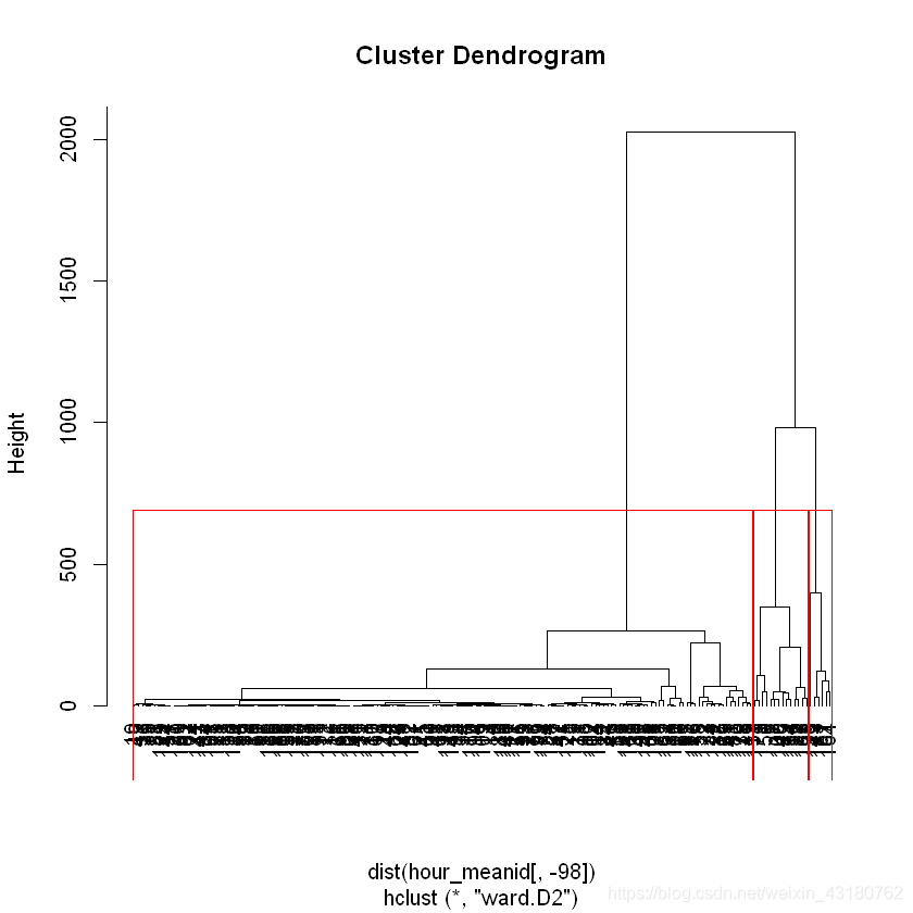
## 系统聚类及可视化
hc1 <- hclust(dist(hour_meanid[,-98]),method = "ward.D2")
##  可视化结果
par(family = "STKaiti",cex = 0.45)
Warning message in dist(hour_meanid[, -98]):
"强制改变过程中产生了NA"
plot(hc1,hang = -1)
rect.hclust(hc1, k=3, border="red")
library(ggplot2)
library(gridExtra)
library(ggdendro)
library(cluster)
library(ggfortify)
ggdendrogram(hc1, segments = T,rotate = F, theme_dendro = FALSE,size = 4)+theme_bw()+theme(axis.text.x = element_text(size = 5,angle = 90))
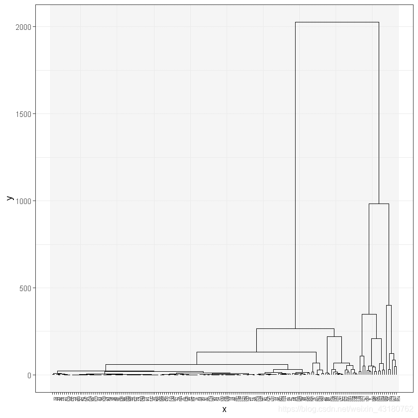
在R中运行,可以得到高清图,因为编译器问题,图片可能比较糊
②K-means聚类
## 计算组内平方和  组间平方和
tot_withinss <- vector()
betweenss <- vector()
for(ii in 1:15){k1 <- kmeans(hour_meanid[,c(-1,-98)],ii)tot_withinss[ii] <- k1$tot.withinssbetweenss[ii] <- k1$betweenss
}kmeanvalue <- data.frame(kk = 1:15,tot_withinss = tot_withinss,betweenss = betweenss)
p1 <- ggplot(kmeanvalue,aes(x = kk,y = tot_withinss))+theme_bw()+geom_point() + geom_line() +labs(y = "value") +ggtitle("Total within-cluster sum of squares")+theme(plot.title = element_text(hjust = 0.5))+scale_x_continuous("kmean 聚类个数",kmeanvalue$kk)p2 <- ggplot(kmeanvalue,aes(x = kk,y = betweenss))+theme_bw()+geom_point() +geom_line() +labs(y = "value") +ggtitle("The between-cluster sum of squares") +theme(plot.title = element_text(hjust = 0.5))+scale_x_continuous("kmean 聚类个数",kmeanvalue$kk)grid.arrange(p1,p2,nrow=2)
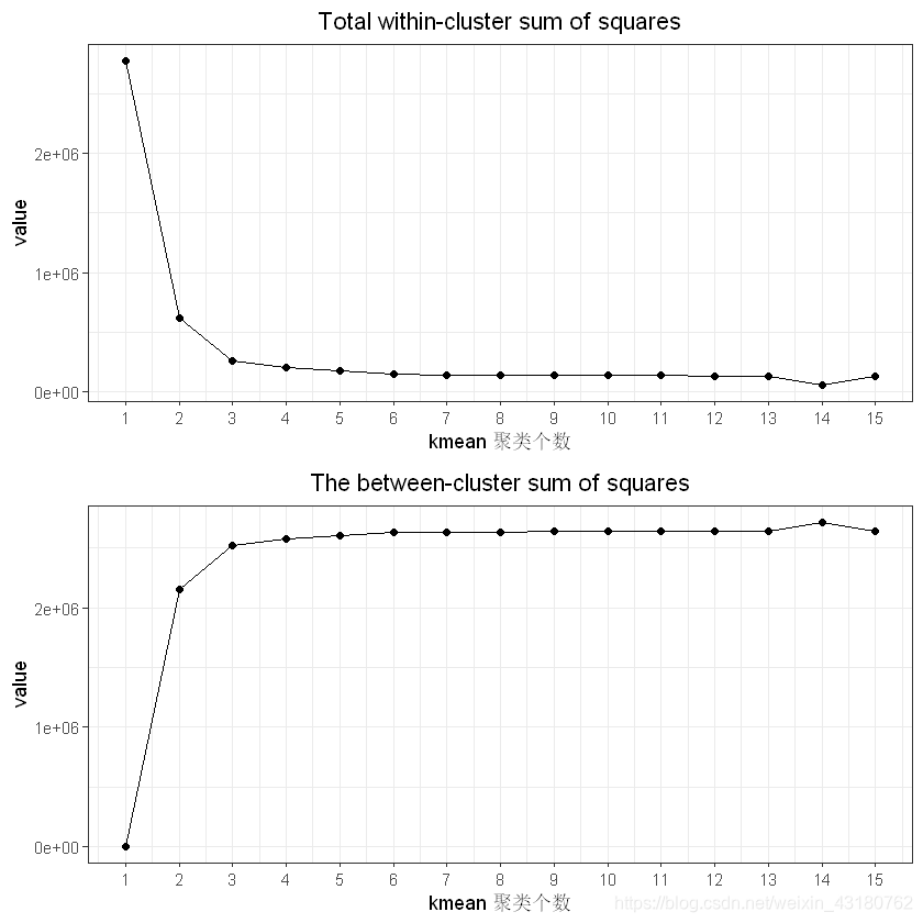
可知,可分为3-4类左右
set.seed(245)
k3 <- kmeans(hour_meanid[,c(-1,-98)],4)
summary(k3)
             Length Class  Mode
cluster      176    -none- numeric
centers      384    -none- numeric
totss          1    -none- numeric
withinss       4    -none- numeric
tot.withinss   1    -none- numeric
betweenss      1    -none- numeric
size           4    -none- numeric
iter           1    -none- numeric
ifault         1    -none- numeric
k3
K-means clustering with 4 clusters of sizes 6, 14, 12, 144Cluster means:00:00-00:15 00:15-00:30 00:30-00:45 00:45-01:00 01:00-01:15 01:15-01:30
1  62.3225417  61.5598583  63.6116083  60.9971833  63.6551667  63.0593333
2  11.0446536  11.1182536  10.5954179  10.9049750  10.8082393  10.9635143
3  27.1211361  27.7766042  27.0752431  27.9496597  27.0779917  28.0800056
4   0.6796588   0.6750685   0.6726699   0.6789852   0.6641741   0.670610901:30-01:45 01:45-02:00 02:00-02:15 02:15-02:30 02:30-02:45 02:45-03:00
1  62.3378667  61.9536917  62.5135250  63.8845000  61.6807417  62.3915167
2  10.8759214  10.8956643  10.7552357  10.9384250  10.8762357  10.7623750
3  27.1717583  27.4775153  27.5150958  27.8758236  27.9836847  27.5832681
4   0.6772897   0.6643105   0.6722411   0.6603515   0.6549296   0.656200503:00-03:15 03:15-03:30 03:30-03:45 03:45-04:00 04:00-04:15 04:15-04:30
1  60.9340500  62.9090583  61.6450583  60.8104000    61.76591  62.3655333
2  10.8683857  11.0325750  10.7480857  10.8762000    10.91756  10.7136857
3  27.7674792  28.0245264  27.7221507  27.6713938    27.59359  27.7191694
4   0.6507282   0.6617699   0.6492977   0.6531032     0.65239   0.6486241
.....Clustering vector:[1] 4 4 2 4 4 3 3 4 3 4 4 4 4 4 4 4 4 4 4 4 4 4 4 4 4 4 4 4 4 4 4 4 4 4 1 4 4[38] 4 4 4 4 4 4 4 4 4 4 4 4 4 4 4 4 4 4 4 4 4 4 4 4 4 4 4 2 4 1 4 2 4 4 4 4 4[75] 4 4 4 4 4 4 4 4 4 4 2 4 2 4 3 4 4 4 4 4 4 4 4 4 4 3 4 4 4 4 4 4 4 4 4 4 4
[112] 4 4 4 4 4 4 2 2 4 4 4 4 4 4 4 4 4 4 4 4 2 4 4 4 4 4 2 4 4 4 4 4 4 4 3 4 4
[149] 1 3 2 4 3 3 4 4 4 2 2 4 1 4 4 1 3 4 4 4 3 2 3 4 1 4 4 2Within cluster sum of squares by cluster:
[1] 91916.57 33987.51 60979.15 15200.70(between_SS / total_SS =  92.7 %)Available components:[1] "cluster"      "centers"      "totss"        "withinss"     "tot.withinss"
[6] "betweenss"    "size"         "iter"         "ifault"
#将标签写入
hour_meanid$cluster<-k3$cluster
head(hour_meanid)
| id | 00:00-00:15 | 00:15-00:30 | 00:30-00:45 | 00:45-01:00 | 01:00-01:15 | 01:15-01:30 | 01:30-01:45 | 01:45-02:00 | 02:00-02:15 | ... | 22:00-22:15 | 22:15-22:30 | 22:30-22:45 | 22:45-23:00 | 23:00-23:15 | 23:15-23:30 | 23:30-23:45 | 23:45-00:00 | rowsum | cluster |
|---|---|---|---|---|---|---|---|---|---|---|---|---|---|---|---|---|---|---|---|---|
| <chr> | <dbl> | <dbl> | <dbl> | <dbl> | <dbl> | <dbl> | <dbl> | <dbl> | <dbl> | ... | <dbl> | <dbl> | <dbl> | <dbl> | <dbl> | <dbl> | <dbl> | <dbl> | <dbl> | <int> |
| 客户10 | 0.45400 | 0.45400 | 0.45400 | 0.45400 | 0.45400 | 0.45400 | 0.45400 | 0.45400 | 0.45400 | ... | 0.45400 | 0.45400 | 0.45400 | 0.45400 | 0.45400 | 0.45400 | 0.45400 | 0.45400 | 44.0320 | 4 |
| 客户100 | 0.28375 | 0.28375 | 0.28375 | 0.28375 | 0.28375 | 0.28375 | 0.28375 | 0.28375 | 0.28375 | ... | 0.63815 | 0.63815 | 0.63815 | 0.63815 | 0.28375 | 0.28375 | 0.28375 | 0.28375 | 67.1776 | 4 |
| 客户101 | 10.69600 | 10.36000 | 9.40800 | 10.41600 | 10.30400 | 10.64000 | 10.36000 | 10.36000 | 9.96800 | ... | 0.00000 | 0.00000 | 0.00000 | 0.00000 | 10.30400 | 10.92000 | 10.02400 | 10.80800 | 327.2640 | 2 |
| 客户102 | 3.08600 | 3.08600 | 3.08600 | 3.08600 | 3.08600 | 3.08600 | 3.08600 | 3.08600 | 3.08600 | ... | 3.08600 | 3.08600 | 3.08600 | 3.08600 | 3.08600 | 3.08600 | 3.08600 | 3.08600 | 299.2640 | 4 |
| 客户103 | 0.83400 | 0.76200 | 0.70200 | 0.80400 | 0.75600 | 0.80700 | 0.73500 | 0.82500 | 0.72300 | ... | 0.78000 | 0.82200 | 0.81000 | 0.82800 | 0.76200 | 0.85200 | 0.77400 | 0.81000 | 75.0780 | 4 |
| 客户104 | 23.31025 | 24.53075 | 21.38475 | 25.41075 | 22.83675 | 24.02475 | 22.11075 | 23.66960 | 23.85660 | ... | 24.26030 | 24.70030 | 24.66730 | 24.66730 | 24.73730 | 20.77730 | 24.73730 | 22.09730 | 2368.3790 | 3 |
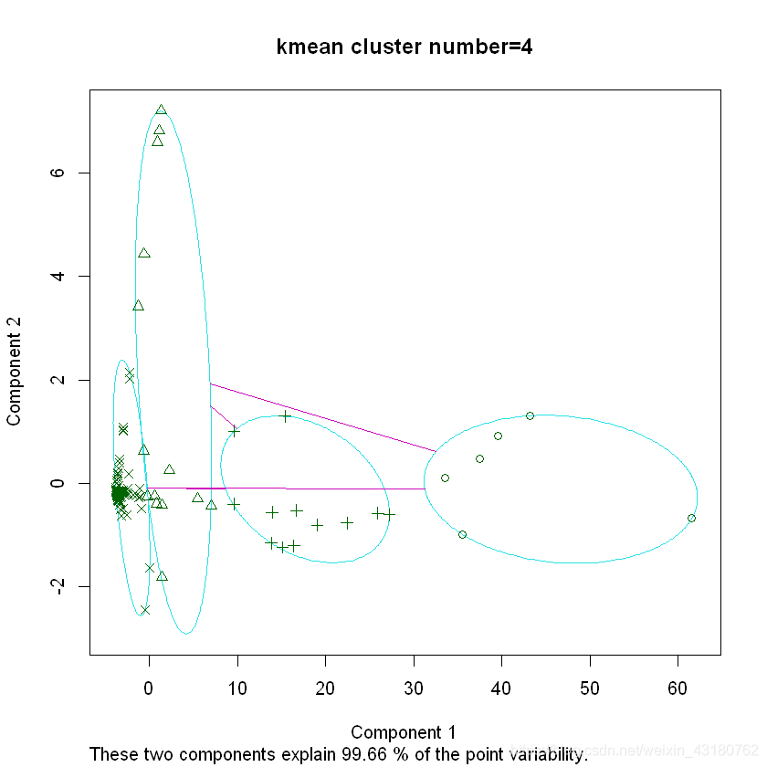
可发现:1,2,3,4类别以此对应电力负荷从大到小,其中1类的电力负荷用量最大,4类负荷小,且大部分用户都是4类,高用电的客户较少,符合常理。
#查看类别分布情况
table(k3$cluster)
1 2 3 4 6 14 12 144
## 对聚类结果可视化
clusplot(hour_meanid[,c(-1,-98)],k3$cluster,main = "kmean cluster number=4")
## 可视化轮廓图,表示聚类效果
sis1 <- silhouette(k3$cluster,dist(hour_meanid[,c(-1,-98)],method = "euclidean"))plot(sis1,main = " kmean silhouette",col = c("red", "green", "blue","orange"))
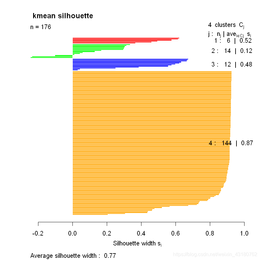
根据可视化,可看出分类合理
最后的分类情况为:
cluster<-hour_meanid[,c(1,98,99)]
head(cluster)
| id | rowsum | cluster |
|---|---|---|
| <chr> | <dbl> | <int> |
| 客户10 | 44.0320 | 4 |
| 客户100 | 67.1776 | 4 |
| 客户101 | 327.2640 | 2 |
| 客户102 | 299.2640 | 4 |
| 客户103 | 75.0780 | 4 |
| 客户104 | 2368.3790 | 3 |
五.构建特征,建立预测模型
#计算每天各时段总功率情况
hour_perdata<-data%>%select(-id)%>% group_by(date)%>%summarise(across(contains(":"),sum,na.rm=TRUE))
head(hour_perdata)
| date | 00:00-00:15 | 00:15-00:30 | 00:30-00:45 | 00:45-01:00 | 01:00-01:15 | 01:15-01:30 | 01:30-01:45 | 01:45-02:00 | 02:00-02:15 | ... | 21:30-21:45 | 21:45-22:00 | 22:00-22:15 | 22:15-22:30 | 22:30-22:45 | 22:45-23:00 | 23:00-23:15 | 23:15-23:30 | 23:30-23:45 | 23:45-00:00 |
|---|---|---|---|---|---|---|---|---|---|---|---|---|---|---|---|---|---|---|---|---|
| <chr> | <dbl> | <dbl> | <dbl> | <dbl> | <dbl> | <dbl> | <dbl> | <dbl> | <dbl> | ... | <dbl> | <dbl> | <dbl> | <dbl> | <dbl> | <dbl> | <dbl> | <dbl> | <dbl> | <dbl> |
| 2020-10-01 | 1072.639 | 1029.341 | 1126.394 | 1006.468 | 1149.825 | 1049.246 | 1081.704 | 1043.298 | 1035.710 | ... | 903.034 | 925.398 | 892.032 | 895.551 | 916.666 | 848.736 | 1061.042 | 1039.832 | 1070.716 | 1108.838 |
| 2020-10-02 | 1053.230 | 1061.432 | 1071.509 | 1066.805 | 1064.543 | 1082.807 | 1077.749 | 1059.869 | 1061.881 | ... | 854.297 | 890.661 | 889.655 | 926.648 | 934.576 | 840.278 | 1080.117 | 1047.243 | 1068.415 | 1046.172 |
| 2020-10-03 | 1066.082 | 1041.977 | 1063.421 | 1035.097 | 1065.615 | 1051.490 | 1083.908 | 1086.658 | 1094.954 | ... | 887.702 | 882.407 | 906.146 | 880.330 | 927.592 | 933.959 | 1020.249 | 1063.968 | 1034.539 | 1070.460 |
| 2020-10-04 | 1020.191 | 1019.630 | 1024.692 | 998.385 | 1051.136 | 1027.053 | 1039.158 | 1028.785 | 1043.948 | ... | 888.178 | 872.275 | 900.867 | 888.164 | 846.700 | 944.616 | 1009.187 | 990.422 | 1063.672 | 1011.367 |
| 2020-10-05 | 1045.160 | 1042.054 | 1027.871 | 1040.656 | 1029.198 | 1024.341 | 1063.339 | 1048.033 | 1053.538 | ... | 949.303 | 986.068 | 1005.798 | 914.553 | 975.165 | 955.135 | 998.024 | 1213.050 | 1093.703 | 1096.247 |
| 2020-10-06 | 1135.002 | 1150.890 | 1084.839 | 1116.269 | 1113.480 | 1106.495 | 1085.247 | 1134.322 | 1125.822 | ... | 889.987 | 898.923 | 866.585 | 919.430 | 972.184 | 913.558 | 1072.352 | 1091.411 | 1104.961 | 1133.166 |
从日期中找到特征,如节假日,周末等
library(tseries)
library(forecast)
Warning message:
"package 'forecast' was built under R version 4.0.4"
Registered S3 methods overwritten by 'forecast':method                 from     autoplot.Arima         ggfortifyautoplot.acf           ggfortifyautoplot.ar            ggfortifyautoplot.bats          ggfortifyautoplot.decomposed.ts ggfortifyautoplot.ets           ggfortifyautoplot.forecast      ggfortifyautoplot.stl           ggfortifyautoplot.ts            ggfortifyfitted.ar              ggfortifyfortify.ts             ggfortifyresiduals.ar           ggfortify
hour_perdata$date<-as.Date(hour_perdata$date)#转为时间格式
library(lubridate)hour_perdata$day<-day(hour_perdata$date)#提取天
hour_perdata$week<-weekdays(as.Date(hour_perdata$date))
head(hour_perdata)| date | 00:00-00:15 | 00:15-00:30 | 00:30-00:45 | 00:45-01:00 | 01:00-01:15 | 01:15-01:30 | 01:30-01:45 | 01:45-02:00 | 02:00-02:15 | ... | 22:45-23:00 | 23:00-23:15 | 23:15-23:30 | 23:30-23:45 | 23:45-00:00 | day | week | week01 | week02 | fes |
|---|---|---|---|---|---|---|---|---|---|---|---|---|---|---|---|---|---|---|---|---|
| <date> | <dbl> | <dbl> | <dbl> | <dbl> | <dbl> | <dbl> | <dbl> | <dbl> | <dbl> | ... | <dbl> | <dbl> | <dbl> | <dbl> | <dbl> | <int> | <chr> | <dbl> | <dbl> | <dbl> |
| 2020-10-01 | 1072.639 | 1029.341 | 1126.394 | 1006.468 | 1149.825 | 1049.246 | 1081.704 | 1043.298 | 1035.710 | ... | 848.736 | 1061.042 | 1039.832 | 1070.716 | 1108.838 | 1 | 星期四 | 0 | 0 | 1 |
| 2020-10-02 | 1053.230 | 1061.432 | 1071.509 | 1066.805 | 1064.543 | 1082.807 | 1077.749 | 1059.869 | 1061.881 | ... | 840.278 | 1080.117 | 1047.243 | 1068.415 | 1046.172 | 2 | 星期五 | 0 | 0 | 1 |
| 2020-10-03 | 1066.082 | 1041.977 | 1063.421 | 1035.097 | 1065.615 | 1051.490 | 1083.908 | 1086.658 | 1094.954 | ... | 933.959 | 1020.249 | 1063.968 | 1034.539 | 1070.460 | 3 | 星期六 | 0 | 1 | 1 |
| 2020-10-04 | 1020.191 | 1019.630 | 1024.692 | 998.385 | 1051.136 | 1027.053 | 1039.158 | 1028.785 | 1043.948 | ... | 944.616 | 1009.187 | 990.422 | 1063.672 | 1011.367 | 4 | 星期日 | 1 | 0 | 1 |
| 2020-10-05 | 1045.160 | 1042.054 | 1027.871 | 1040.656 | 1029.198 | 1024.341 | 1063.339 | 1048.033 | 1053.538 | ... | 955.135 | 998.024 | 1213.050 | 1093.703 | 1096.247 | 5 | 星期一 | 0 | 0 | 1 |
| 2020-10-06 | 1135.002 | 1150.890 | 1084.839 | 1116.269 | 1113.480 | 1106.495 | 1085.247 | 1134.322 | 1125.822 | ... | 913.558 | 1072.352 | 1091.411 | 1104.961 | 1133.166 | 6 | 星期二 | 0 | 0 | 1 |
#将是否周末的信息二值化
hour_perdata$week01 <- ifelse(hour_perdata$week =="星期日" ,1,0)
hour_perdata$week02 <- ifelse(hour_perdata$week =="星期六" ,1,0)
#head(hour_perdata)
#将节假日二值化,比如10.1-10.8是国庆节
hour_perdata$fes <- ifelse(hour_perdata$day <=8 ,1,0)
head(hour_perdata)
| date | 00:00-00:15 | 00:15-00:30 | 00:30-00:45 | 00:45-01:00 | 01:00-01:15 | 01:15-01:30 | 01:30-01:45 | 01:45-02:00 | 02:00-02:15 | ... | 22:45-23:00 | 23:00-23:15 | 23:15-23:30 | 23:30-23:45 | 23:45-00:00 | day | week | week01 | week02 | fes |
|---|---|---|---|---|---|---|---|---|---|---|---|---|---|---|---|---|---|---|---|---|
| <date> | <dbl> | <dbl> | <dbl> | <dbl> | <dbl> | <dbl> | <dbl> | <dbl> | <dbl> | ... | <dbl> | <dbl> | <dbl> | <dbl> | <dbl> | <int> | <chr> | <dbl> | <dbl> | <dbl> |
| 2020-10-01 | 1072.639 | 1029.341 | 1126.394 | 1006.468 | 1149.825 | 1049.246 | 1081.704 | 1043.298 | 1035.710 | ... | 848.736 | 1061.042 | 1039.832 | 1070.716 | 1108.838 | 1 | 星期四 | 0 | 0 | 1 |
| 2020-10-02 | 1053.230 | 1061.432 | 1071.509 | 1066.805 | 1064.543 | 1082.807 | 1077.749 | 1059.869 | 1061.881 | ... | 840.278 | 1080.117 | 1047.243 | 1068.415 | 1046.172 | 2 | 星期五 | 0 | 0 | 1 |
| 2020-10-03 | 1066.082 | 1041.977 | 1063.421 | 1035.097 | 1065.615 | 1051.490 | 1083.908 | 1086.658 | 1094.954 | ... | 933.959 | 1020.249 | 1063.968 | 1034.539 | 1070.460 | 3 | 星期六 | 0 | 1 | 1 |
| 2020-10-04 | 1020.191 | 1019.630 | 1024.692 | 998.385 | 1051.136 | 1027.053 | 1039.158 | 1028.785 | 1043.948 | ... | 944.616 | 1009.187 | 990.422 | 1063.672 | 1011.367 | 4 | 星期日 | 1 | 0 | 1 |
| 2020-10-05 | 1045.160 | 1042.054 | 1027.871 | 1040.656 | 1029.198 | 1024.341 | 1063.339 | 1048.033 | 1053.538 | ... | 955.135 | 998.024 | 1213.050 | 1093.703 | 1096.247 | 5 | 星期一 | 0 | 0 | 1 |
| 2020-10-06 | 1135.002 | 1150.890 | 1084.839 | 1116.269 | 1113.480 | 1106.495 | 1085.247 | 1134.322 | 1125.822 | ... | 913.558 | 1072.352 | 1091.411 | 1104.961 | 1133.166 | 6 | 星期二 | 0 | 0 | 1 |
#write_csv(hour_perdata,"hour_perdata.csv")
①预测未来一天,各时段的电力负荷
#将时间表转置
hour_perdatat<-t(hour_perdata)
hour_perdatat<-as.data.frame(hour_perdatat)
colnames(hour_perdatat)<-hour_perdatat[1,]
hour_perdatat<-hour_perdatat[-1,]
#hour_perdatat$hour<-rownames(hour_perdatat)
#rownames(hour_perdatat)<-c(1:96)
#head(hour_perdatat)
#更改列名
rownames(hour_perdatat)<-hour_perdatat[,21]
head(hour_perdatat)
| 2020-10-01 | 2020-10-02 | 2020-10-03 | 2020-10-04 | 2020-10-05 | 2020-10-06 | 2020-10-07 | 2020-10-08 | 2020-10-09 | 2020-10-10 | ... | 2020-10-12 | 2020-10-13 | 2020-10-14 | 2020-10-15 | 2020-10-16 | 2020-10-17 | 2020-10-18 | 2020-10-19 | 2020-10-20 | hour | |
|---|---|---|---|---|---|---|---|---|---|---|---|---|---|---|---|---|---|---|---|---|---|
| <chr> | <chr> | <chr> | <chr> | <chr> | <chr> | <chr> | <chr> | <chr> | <chr> | ... | <chr> | <chr> | <chr> | <chr> | <chr> | <chr> | <chr> | <chr> | <chr> | <chr> | |
| 00:00-00:15 | 1072.639 | 1053.230 | 1066.082 | 1020.191 | 1045.160 | 1135.002 | 1137.515 | 1152.525 | 1067.732 | 994.568 | ... | 1151.424 | 1110.697 | 1115.400 | 1212.665 | 1165.643 | 1182.825 | 1135.229 | 1150.423 | 1071.966 | 00:00-00:15 |
| 00:15-00:30 | 1029.341 | 1061.432 | 1041.977 | 1019.630 | 1042.054 | 1150.890 | 1184.908 | 1133.851 | 1065.854 | 956.716 | ... | 1199.721 | 1162.543 | 1110.875 | 1141.027 | 1207.853 | 1162.515 | 1105.980 | 1180.014 | 1121.971 | 00:15-00:30 |
| 00:30-00:45 | 1126.394 | 1071.509 | 1063.421 | 1024.692 | 1027.871 | 1084.839 | 1106.957 | 1172.472 | 995.550 | 950.803 | ... | 1120.132 | 1151.471 | 1130.677 | 1203.013 | 1201.945 | 1197.636 | 1152.169 | 1163.545 | 1093.053 | 00:30-00:45 |
| 00:45-01:00 | 1006.468 | 1066.805 | 1035.097 | 998.385 | 1040.656 | 1116.269 | 1157.146 | 1102.331 | 1095.603 | 1008.611 | ... | 1159.193 | 1169.906 | 1062.571 | 1165.559 | 1151.602 | 1166.322 | 1193.887 | 1174.572 | 1171.423 | 00:45-01:00 |
| 01:00-01:15 | 1149.825 | 1064.543 | 1065.615 | 1051.136 | 1029.198 | 1113.480 | 1092.436 | 1127.408 | 1033.743 | 961.246 | ... | 1204.588 | 1095.289 | 1152.565 | 1192.592 | 1277.848 | 1084.228 | 1141.221 | 1189.006 | 1062.351 | 01:00-01:15 |
| 01:15-01:30 | 1049.246 | 1082.807 | 1051.490 | 1027.053 | 1024.341 | 1106.495 | 1175.856 | 1156.887 | 1083.512 | 1037.840 | ... | 1198.193 | 1125.723 | 1120.467 | 1232.879 | 1196.588 | 1169.740 | 1212.220 | 1192.188 | 1125.762 | 01:15-01:30 |
#write_csv(hour_perdatat,"hour_perdatat.csv")
#导入整理后数据
timedata<- read.csv("hour_perdatat.csv",,encoding='UTF-8')
head(timedata)
| hour | sum | |
|---|---|---|
| <chr> | <dbl> | |
| 1 | 00:00-00:15 | 1072.639 |
| 2 | 00:15-00:30 | 1029.341 |
| 3 | 00:30-00:45 | 1126.394 |
| 4 | 00:45-01:00 | 1006.468 |
| 5 | 01:00-01:15 | 1149.825 |
| 6 | 01:15-01:30 | 1049.246 |
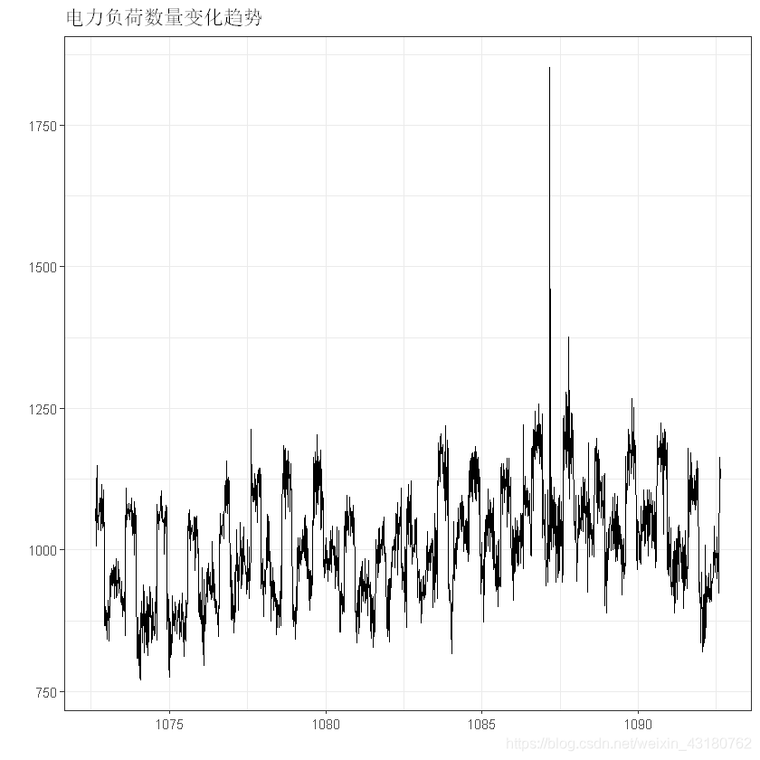
timedata$sum<- ts(timedata$sum,start = timedata$sum[1],frequency = 96)
## 可视化序列
autoplot(timedata$sum)+ggtitle("电力负荷数量变化趋势")
auto.arima(timedata$sum)
Series: timedata$sum
ARIMA(4,1,2)(0,1,0)[96] Coefficients:ar1      ar2      ar3      ar4      ma1      ma2-0.9814  -0.3626  -0.1371  -0.0666  -0.0126  -0.3784
s.e.   0.2001   0.1060   0.0771   0.0390   0.1994   0.1503sigma^2 estimated as 3525:  log likelihood=-10028.98
AIC=20071.97   AICc=20072.03   BIC=20110.52
## 白噪声检验
Box.test(timedata$sum,type ="Ljung-Box")
	Box-Ljung testdata:  timedata$sum
X-squared = 1198.6, df = 1, p-value < 2.2e-16
p-value < 2.2e-16,说明不是白噪声
## 平稳性检验,单位根检验
adf.test(timedata$sum)
Warning message in adf.test(timedata$sum):
"p-value smaller than printed p-value"Augmented Dickey-Fuller Testdata:  timedata$sum
Dickey-Fuller = -8.312, Lag order = 12, p-value = 0.01
alternative hypothesis: stationary
p-value = 0.01,说明数据是平稳的
由之前自动建模可知适合的模型为:
Series: timedata$sum
ARIMA(4,1,2)(0,1,0)[96]
Coefficients:
ar1 ar2 ar3 ar4 ma1 ma2
-0.9814 -0.3626 -0.1371 -0.0666 -0.0126 -0.3784
s.e. 0.2001 0.1060 0.0771 0.0390 0.1994 0.1503
sigma^2 estimated as 3525: log likelihood=-10028.98
AIC=20071.97 AICc=20072.03 BIC=20110.52
## 对数据建立ARIMA(4,1,2)(0,1,0)[96]模型,并预测后面的数据ARIMA <- arima(timedata$sum, c(4, 1, 2),seasonal = list(order = c(0, 1, 0),period = 96))
summary(ARIMA)
Call:
arima(x = timedata$sum, order = c(4, 1, 2), seasonal = list(order = c(0, 1, 0), period = 96))Coefficients:ar1      ar2      ar3      ar4      ma1      ma2-0.9814  -0.3626  -0.1371  -0.0666  -0.0126  -0.3784
s.e.   0.2001   0.1060   0.0771   0.0390   0.1994   0.1503sigma^2 estimated as 3513:  log likelihood = -10028.98,  aic = 20071.97Training set error measures:ME     RMSE      MAE        MPE     MAPE      MASE
Training set 0.09120194 57.75377 39.33659 -0.1172248 3.877619 0.9060558ACF1
Training set 0.0008442811
Box.test(ARIMA$residuals,type ="Ljung-Box")
## p-value = 0.9705,此时,模型的残差已经是白噪声数据,数据中的信息已经充分的提取出来了
	Box-Ljung testdata:  ARIMA$residuals
X-squared = 0.0013707, df = 1, p-value = 0.9705
p-value = 0.9705,此时,模型的残差已经是白噪声数据,数据中的信息已经充分的提取出来了
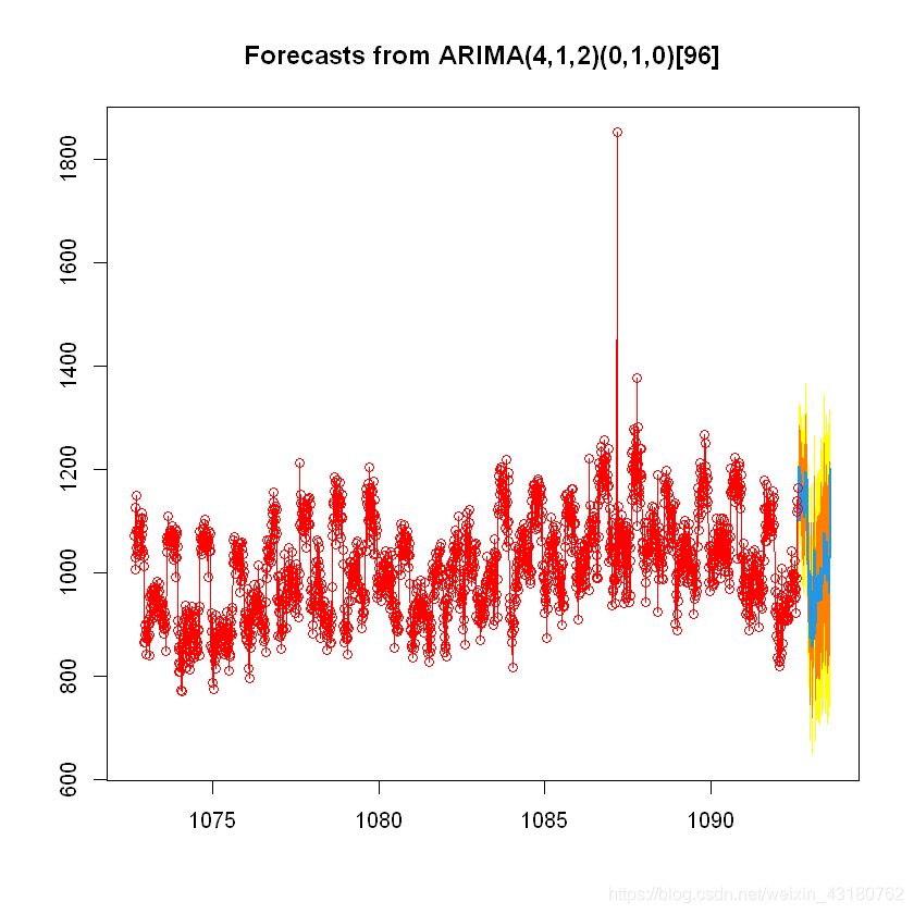
# 可视化模型的预测值和这是值之间的差距
par(family = "STKaiti")
plot(forecast(ARIMA,h=96),shadecols="oldstyle")
points(timedata$sum,col = "red")
lines(timedata$sum,col = "red")
#输出未来一天的预测值
fore<-as.data.frame(forecast(ARIMA,h=96))
head(fore)
| Point Forecast | Lo 80 | Hi 80 | Lo 95 | Hi 95 | |
|---|---|---|---|---|---|
| <dbl> | <dbl> | <dbl> | <dbl> | <dbl> | |
| 1092.639 | 1098.481 | 1022.523 | 1174.438 | 982.3139 | 1214.648 |
| 1092.649 | 1155.922 | 1079.964 | 1231.881 | 1039.7534 | 1272.091 |
| 1092.660 | 1133.867 | 1055.742 | 1211.992 | 1014.3850 | 1253.349 |
| 1092.670 | 1206.424 | 1126.309 | 1286.539 | 1083.8980 | 1328.950 |
| 1092.681 | 1102.090 | 1020.172 | 1184.008 | 976.8067 | 1227.373 |
| 1092.691 | 1161.522 | 1077.076 | 1245.969 | 1032.3722 | 1290.673 |
label<-as.data.frame(rownames(hour_perdatat))
label<-label[c(-101,-100,-99,-98,-97),]
fore$label<-label
rownames(fore)<-fore$label
fore
| Point Forecast | Lo 80 | Hi 80 | Lo 95 | Hi 95 | label | |
|---|---|---|---|---|---|---|
| <dbl> | <dbl> | <dbl> | <dbl> | <dbl> | <chr> | |
| 00:00-00:15 | 1098.4808 | 1022.5234 | 1174.438 | 982.3139 | 1214.648 | 00:00-00:15 |
| 00:15-00:30 | 1155.9223 | 1079.9635 | 1231.881 | 1039.7534 | 1272.091 | 00:15-00:30 |
| 00:30-00:45 | 1133.8668 | 1055.7419 | 1211.992 | 1014.3850 | 1253.349 | 00:30-00:45 |
| 00:45-01:00 | 1206.4239 | 1126.3085 | 1286.539 | 1083.8980 | 1328.950 | 00:45-01:00 |
| 01:00-01:15 | 1102.0896 | 1020.1716 | 1184.008 | 976.8067 | 1227.373 | 01:00-01:15 |
| 01:15-01:30 | 1161.5225 | 1077.0756 | 1245.969 | 1032.3722 | 1290.673 | 01:15-01:30 |
| 01:30-01:45 | 1191.8077 | 1105.8064 | 1277.809 | 1060.2800 | 1323.335 | 01:30-01:45 |
| 01:45-02:00 | 1127.9435 | 1039.7995 | 1216.088 | 993.1389 | 1262.748 | 01:45-02:00 |
| 02:00-02:15 | 1120.8414 | 1030.9879 | 1210.695 | 983.4223 | 1258.260 | 02:00-02:15 |
| 02:15-02:30 | 1163.5182 | 1071.7734 | 1255.263 | 1023.2066 | 1303.830 | 02:15-02:30 |
| 02:30-02:45 | 1118.0552 | 1024.5597 | 1211.551 | 975.0661 | 1261.044 | 02:30-02:45 |
| 02:45-03:00 | 1135.7189 | 1040.4717 | 1230.966 | 990.0510 | 1281.387 | 02:45-03:00 |
| 03:00-03:15 | 1141.9914 | 1045.0253 | 1238.957 | 993.6945 | 1290.288 | 03:00-03:15 |
| 03:15-03:30 | 1124.3686 | 1025.7242 | 1223.013 | 973.5051 | 1275.232 | 03:15-03:30 |
| 03:30-03:45 | 1165.7177 | 1065.4104 | 1266.025 | 1012.3110 | 1319.124 | 03:30-03:45 |
| 03:45-04:00 | 1168.6668 | 1066.7342 | 1270.599 | 1012.7743 | 1324.559 | 03:45-04:00 |
| 04:00-04:15 | 1117.2710 | 1013.7314 | 1220.811 | 958.9209 | 1275.621 | 04:00-04:15 |
| 04:15-04:30 | 1159.8146 | 1054.6969 | 1264.932 | 999.0509 | 1320.578 | 04:15-04:30 |
| 04:30-04:45 | 1108.2668 | 1001.5921 | 1214.941 | 945.1220 | 1271.412 | 04:30-04:45 |
| 04:45-05:00 | 1143.0876 | 1034.8792 | 1251.296 | 977.5971 | 1308.578 | 04:45-05:00 |
| 05:00-05:15 | 1116.9023 | 1007.1815 | 1226.623 | 949.0988 | 1284.706 | 05:00-05:15 |
| 05:15-05:30 | 1167.5618 | 1056.3490 | 1278.775 | 997.4765 | 1337.647 | 05:15-05:30 |
| 05:30-05:45 | 1194.9829 | 1082.2980 | 1307.668 | 1022.6462 | 1367.320 | 05:30-05:45 |
| 05:45-06:00 | 1125.4082 | 1011.2701 | 1239.546 | 950.8490 | 1299.967 | 05:45-06:00 |
| 06:00-06:15 | 1178.4606 | 1062.8876 | 1294.034 | 1001.7070 | 1355.214 | 06:00-06:15 |
| 06:15-06:30 | 1131.3154 | 1014.3251 | 1248.306 | 952.3942 | 1310.237 | 06:15-06:30 |
| 06:30-06:45 | 1181.8554 | 1063.4649 | 1300.246 | 1000.7927 | 1362.918 | 06:30-06:45 |
| 06:45-07:00 | 1130.1775 | 1010.4029 | 1249.952 | 946.9981 | 1313.357 | 06:45-07:00 |
| 07:00-07:15 | 1026.6404 | 905.4977 | 1147.783 | 841.3687 | 1211.912 | 07:00-07:15 |
| 07:15-07:30 | 962.4825 | 839.9869 | 1084.978 | 775.1417 | 1149.823 | 07:15-07:30 |
| ... | ... | ... | ... | ... | ... | ... |
| 16:30-16:45 | 1011.7984 | 846.8720 | 1176.725 | 759.5652 | 1264.032 | 16:30-16:45 |
| 16:45-17:00 | 951.7214 | 785.7988 | 1117.644 | 697.9646 | 1205.478 | 16:45-17:00 |
| 17:00-17:15 | 947.1024 | 780.1895 | 1114.015 | 691.8311 | 1202.374 | 17:00-17:15 |
| 17:15-17:30 | 980.5094 | 812.6120 | 1148.407 | 723.7324 | 1237.286 | 17:15-17:30 |
| 17:30-17:45 | 983.0574 | 814.1813 | 1151.934 | 724.7836 | 1241.331 | 17:30-17:45 |
| 17:45-18:00 | 979.1334 | 809.2842 | 1148.983 | 719.3714 | 1238.895 | 17:45-18:00 |
| 18:00-18:15 | 995.6674 | 824.8506 | 1166.484 | 734.4257 | 1256.909 | 18:00-18:15 |
| 18:15-18:30 | 1012.9484 | 841.1695 | 1184.727 | 750.2353 | 1275.662 | 18:15-18:30 |
| 18:30-18:45 | 1025.9084 | 853.1728 | 1198.644 | 761.7321 | 1290.085 | 18:30-18:45 |
| 18:45-19:00 | 1042.0334 | 868.3463 | 1215.721 | 776.4019 | 1307.665 | 18:45-19:00 |
| 19:00-19:15 | 1079.0614 | 904.4280 | 1253.695 | 811.9827 | 1346.140 | 19:00-19:15 |
| 19:15-19:30 | 1010.4204 | 834.8459 | 1185.995 | 741.9023 | 1278.939 | 19:15-19:30 |
| 19:30-19:45 | 1034.4144 | 857.9037 | 1210.925 | 764.4646 | 1304.364 | 19:30-19:45 |
| 19:45-20:00 | 997.5734 | 820.1315 | 1175.015 | 726.1994 | 1268.948 | 19:45-20:00 |
| 20:00-20:15 | 1036.5914 | 858.2231 | 1214.960 | 763.8006 | 1309.382 | 20:00-20:15 |
| 20:15-20:30 | 1030.1404 | 850.8505 | 1209.430 | 755.9402 | 1304.341 | 20:15-20:30 |
| 20:30-20:45 | 1031.2764 | 851.0697 | 1211.483 | 755.6740 | 1306.879 | 20:30-20:45 |
| 20:45-21:00 | 1014.4834 | 833.3644 | 1195.602 | 737.4858 | 1291.481 | 20:45-21:00 |
| 21:00-21:15 | 1060.6284 | 878.6018 | 1242.655 | 782.2427 | 1339.014 | 21:00-21:15 |
| 21:15-21:30 | 986.6754 | 803.7456 | 1169.605 | 706.9085 | 1266.442 | 21:15-21:30 |
| 21:30-21:45 | 1031.7954 | 847.9669 | 1215.624 | 750.6540 | 1312.937 | 21:30-21:45 |
| 21:45-22:00 | 1006.3614 | 821.6386 | 1191.084 | 723.8522 | 1288.871 | 21:45-22:00 |
| 22:00-22:15 | 1007.0594 | 821.4466 | 1192.672 | 723.1890 | 1290.930 | 22:00-22:15 |
| 22:15-22:30 | 992.1524 | 805.6538 | 1178.651 | 706.9273 | 1277.378 | 22:15-22:30 |
| 22:30-22:45 | 960.7194 | 773.3392 | 1148.100 | 674.1461 | 1247.293 | 22:30-22:45 |
| 22:45-23:00 | 1027.5134 | 839.2557 | 1215.771 | 739.5981 | 1315.429 | 22:45-23:00 |
| 23:00-23:15 | 1176.6744 | 987.5433 | 1365.806 | 887.4234 | 1465.926 | 23:00-23:15 |
| 23:15-23:30 | 1156.0004 | 965.9999 | 1346.001 | 865.4197 | 1446.581 | 23:15-23:30 |
| 23:30-23:45 | 1201.3474 | 1010.4815 | 1392.213 | 909.4432 | 1493.252 | 23:30-23:45 |
| 23:45-00:00 | 1162.6794 | 970.9520 | 1354.407 | 869.4576 | 1455.901 | 23:45-00:00 |
预测结果如上
②预测未来几天总体电力负荷
可结合周末,季节,月份,年份,节假日,温度等信息,进行建模,利用支持向量机,随机森林或线性模型等建立回归模型,对某天的总额进行预测建模。
由于本例数据为10.01-10.20,时间跨度短,且数据量较小,从理论上讲,预测结果不会太好,故考虑以其他方法进行建模,如回归分析,灰色预测等
#根据按天统计的电力负荷量可得
date_rowsum
plot(date_rowsum,type = "o", col = "red", xlab = "date", ylab = "sum",main = "date_sum")
| date | sum |
|---|---|
| <date> | <dbl> |
| 2020-10-01 | 93125.13 |
| 2020-10-02 | 89564.60 |
| 2020-10-03 | 89715.30 |
| 2020-10-04 | 91119.79 |
| 2020-10-05 | 95884.30 |
| 2020-10-06 | 95558.53 |
| 2020-10-07 | 97199.34 |
| 2020-10-08 | 97358.87 |
| 2020-10-09 | 91890.29 |
| 2020-10-10 | 94850.10 |
| 2020-10-11 | 95424.02 |
| 2020-10-12 | 100501.56 |
| 2020-10-13 | 100307.05 |
| 2020-10-14 | 101899.14 |
| 2020-10-15 | 105264.88 |
| 2020-10-16 | 105435.29 |
| 2020-10-17 | 100331.14 |
| 2020-10-18 | 103870.77 |
| 2020-10-19 | 99513.48 |
| 2020-10-20 | 95456.16 |

在以“天”的维度上,由于国庆节假日影响,不能看出明显的规律,但能看出存在一定周期性,不适用回归模型和灰色预测。
如果需要精确到客户,则提取每个客户每天各时段的数据,套用上述模型即可得到。
但由于单个客户随机性极强,且个人用电较小,细致分析意义不大,可针对高耗电用户进行分析。其余从宏观角度预测以进行电力调配即可。


![[负荷预测]基于线性回归模型的中长期电力负荷预测](https://img-blog.csdnimg.cn/9225bb87e6ba4905be02cd0cd6127e36.png)