1 什么是vintage分析?
Vintage分析(账龄分析法)被广泛应用于信用卡及信贷行业,这个概念起源于葡萄酒,即不同年份出产的葡萄酒的品质有差异,那么不同时期开户或者放款的资产质量也有差异,其核心在于,对不同时期不同批次的资产分别跟踪,按照账龄同步对比,从而能够了解不同时期放款或发行信用卡的资产质量情况。
vintage分析从更广泛的意义来讲属于同期群分析,跟社会跟踪调查、人口学的队列分析技术,互联网运营的留存分析是类似的,具体概念不再赘述。我们直接进入主题,如何使用R语言creditmodel包做Vintage分析。
2 creditmodel包的cohort analysis模块简介
creditmodel是汉森老师开发的一个强大的R语言数据科学工具包,有数据预处理、变量衍生、数据分析、数据可视化、自动化建模五大功能模块。而今天所讲的vintage分析是creditmodel包数据分析模块的一个子模块,包括cohort_analysis、cohort_table、cohort_table_plot、cohort_plot四个主要函数。
3 cohort analysis 模块简介
Description
cohort_analysis cohort_analysis is for cohort(vintage) analysis.
Usage
cohort_analysis(dat, obs_id = NULL, occur_time = NULL, MOB = NULL,period = "monthly", status = NULL, amount = NULL, by_out = "cnt",start_date = NULL, end_date = NULL, dead_status = 30)cohort_table(dat, obs_id = NULL, occur_time = NULL, MOB = NULL,period = "monthly", status = NULL, amount = NULL, by_out = "cnt",start_date = NULL, end_date = NULL, dead_status = 30)
Arguments
dat | A data.frame contained id, occur_time, mob, status … |
|---|---|
obs_id | The name of ID of observations or key variable of data. Default is NULL. |
occur_time | The name of the variable that represents the time at which each observation takes place. |
MOB | Mobility of book |
period | Period of event to analysis. Default is “monthly” |
status | Status of observations |
amount | The name of variable representing amount. Default is NULL. |
by_out | Output: amount (amt) or count (cnt) |
start_date | The earliest occurrence time of observations. |
end_date | The latest occurrence time of observations. |
dead_status | Status of dead observations. |
4 使用vintage分析步骤
4.1 数据准备
进行vintage分析,输入的数据至少要有放款编号(loan_id), 放款时间(loan_time)、放款金额(loan_amount)和账户状态(max_overdue_days或age_overdue_days)四列。
#安装和加载creditmodel包
#install.packages("creditmodel")
library(creditmodel)
#使用read_data读入数据。
vin_dat = read_data("vin_dat.csv")
#使用creditmodel包的数据清晰模块主函数对数据进行清洗,关于数据清洗模块,以后会做详细接受,在此简单描述下各个参数的含义。
vin_dat = data_cleansing(vin_dat, obs_id = "loan_id",#主键occur_time = 'loan_time',#事件发生时间outlier_proc = FALSE,#不进行异常值处理missing_proc = FALSE,#不进行确实值处理remove_dup = FALSE,#不删除重复观测merge_cat = FALSE,#不对类别变量的类别进行合并low_var = 0.9999,#删除单一值比例大于0.9999的变量missing_rate = 0.9999 # 对缺失值比例大于0.9999的变量进行二值化处理)
#可使用creditmodel包的data_exploration函数来观察数据概貌
data_exploration(vin_dat)
>
* Observations      : 204697
* Numeric_variables : 7
* Category_variables: 1
* Date_variables    : 1
$numFeature  NMiss Miss_Rate        Max        75%     Median        25%        Min       Mean   Std
1   age_overdue_days 194695    95.11%        440        122         61         30          1         90    76
2 age_overdue_period     33     0.02%         15          0          0          0          0          0  0.87
3           loan_age     33     0.02%         15          6          3          1          0          4   3.2
4        loan_amount      0        0%     500000      60000      40000      30000       1000      47911 24279
5       loan_balance    823      0.4%     500000      53186      39046      27871        920      43112 22157
6          loan_time      0        0% 2017-09-30 2017-03-31 2016-12-29 2016-11-01 2016-06-01 2017-01-11    99
7   max_overdue_days 160974    78.64%        440         13          2          1          1         23    52
8 max_overdue_period      0        0%       15.0        0.0        0.0        0.0        0.0        0.3  0.93$charFeature  NMiss Miss_Rate                 Value1                 Value2              Value3              Value4              Value5              Value6
1 loan_id 204697      100% n2016060100000030 : 48 n2016060100000010 : 30 n1605300032102 : 16 n1606010034102 : 16 n1606020032402 : 16 n1606020034202 : 16Value7
1 (Other) : 204555
>
#使用plot_table画出数值型变量的数据概要
plot_table(data_exploration(vin_dat)$num)

4.2 vintage分析
4.2.1 cohort_dat表的构建
使用cohort_analysis函数来构建cohort_dat表。
cohort_dat = cohort_analysis(vin_dat,obs_id = 'loan_id',#放款编号occur_time = 'loan_time', #放款时间MOB = NULL,#month on book在账月份,找个可以自己定义为一个变量,默认以自然月为月份。period = 'monthly',#以月作为同一时期,也可按周weeklystatus = "age_overdue_days",#使用账龄末逾期天数作为状态,也为自己定义的0、1变量dead_status = 30, #逾期天数大于30天则为dead状态,若为0、1变量,此处应设为0.amount = "loan_amount", #如果以金额统计,则必须设置,此处按放款金额计算,也可以按余额by_out = 'amt',#如果以金额统计则为‘amt’,以笔数统计则为‘cnt’start_date = "2016-08-01",#统计日开始时间end_date = '2017-05-31'#统计日结束时间)
最终表结构如下:
| Group | Age | Total | Events | Opening | final_Events | Current_rate | Events_rate | Retention_rate |
|---|---|---|---|---|---|---|---|---|
| 2016/8/1 | 0 | 647 | 6 | 647 | 101 | 0.1561 | 0.0093 | 1 |
| 2016/8/1 | 1 | 646 | 21 | 647 | 101 | 0.1561 | 0.0325 | 0.9985 |
| 2016/8/1 | 2 | 645 | 21 | 647 | 101 | 0.1561 | 0.0325 | 0.9969 |
| 2016/8/1 | 3 | 642 | 25 | 647 | 101 | 0.1561 | 0.0386 | 0.9923 |
| 2016/8/1 | 4 | 638 | 33 | 647 | 101 | 0.1561 | 0.051 | 0.9861 |
| 2016/8/1 | 5 | 630 | 47 | 647 | 101 | 0.1561 | 0.0726 | 0.9737 |
4.2.2 画出vintage图
画出vintage图,特别简单,直接使用cohort_plot函数,输入上一步计算的cohort_dat即可。
cohort_plot(cohort_dat)

4.2.3 vintage表格
使用cohort_table函数得到vintage表格,其入参与cohort_analysis 入参完全一致。
vin_table = cohort_table(vin_dat, obs_id = 'loan_id', occur_time = 'loan_time', MOB = NULL,period = 'monthly', status = "max_overdue_days",dead_status = 30, amount = "loan_balance", by_out = 'amt',start_date = "2016-09-01", end_date = '2017-07-31')
最终表格如下表所示:
| Cohort_Group | 1 | 2 | 3 | 4 | 5 | 6 | 7 | 8 | 9 | 10 | 11 | 12 |
|---|---|---|---|---|---|---|---|---|---|---|---|---|
| 2016/9/1 | 0% | 0.48% | 1.19% | 2.09% | 2.78% | 4.11% | 4.46% | 5.45% | 6.06% | 7.67% | 8.43% | 9.47% |
| 2016/10/1 | 0% | 0.34% | 1.37% | 2.61% | 4.03% | 4.50% | 6.27% | 7.04% | 8.31% | 9.19% | 10.70% | |
| 2016/11/1 | 0% | 0.47% | 1.39% | 2.44% | 3.44% | 4.96% | 5.97% | 6.91% | 7.93% | 9.23% | ||
| 2016/12/1 | 0% | 0.39% | 1.37% | 2.07% | 3.25% | 4.29% | 4.60% | 6.18% | 7.39% | |||
| 2017/1/1 | 0% | 0.32% | 0.82% | 1.83% | 2.66% | 3.21% | 4.71% | 5.31% | ||||
| 2017/2/1 | 0% | 0.35% | 1.25% | 2.49% | 2.97% | 5.09% | 7.03% | |||||
| 2017/3/1 | 0% | 0.60% | 1.21% | 1.63% | 4.07% | 5.55% | ||||||
| 2017/4/1 | 0% | 0.16% | 0.83% | 2.81% | 4.52% | |||||||
| 2017/5/1 | 0% | 0.29% | 1.26% | 1.87% | ||||||||
| 2017/6/1 | 0% | 0.47% | 1.27% | |||||||||
| 2017/7/1 | 0% | 0.32% |
4.2.4 画出vintage表格
如何优雅地画出vintage表格呢?本来只需要一步:cohort_table_plot(cohort_dat)即可,但由于汉森老师粗心大意,R语言CRAN库最新的creditmodel1.1.8版本的该函数有一些bug,不能一步画出来,因此我把修复了bug的源码贴出来,在画vintage表格前先加载这个函数。
#' cohort_table_plot
#' \code{cohort_table_plot} is for ploting cohort(vintage) analysis table.
#' @param cohort_dat  A data.frame generated by \code{cohort_analysis}.
#' @import ggplot2
#' @export
cohort_table_plot = function(cohort_dat) {#set global variablesopt = options('warn' = -1, scipen = 200, stringsAsFactors = FALSE, digits = 6) #cohort_dat[is.na(cohort_dat)] = 0#initial parametersCohort_Group = Cohort_Period = Events = Events_rate = Opening_Total = Retention_Total = cohor_dat = final_Events = m_a = max_age = NULL#plotcohort_plot = ggplot(cohort_dat, aes(reorder(paste0(Cohort_Period), Cohort_Period),Cohort_Group, fill = Events_rate)) +geom_tile(colour = 'white') +geom_text(aes(label = as_percent(Events_rate, 4)), size = 3) +scale_fill_gradient2(limits = c(0, max(cohort_dat$Events_rate)),low = love_color('deep_red'), mid = 'white',high = love_color(),midpoint = median(cohort_dat$Events_rate,na.rm = TRUE), na.value = love_color('pale_grey')) +scale_y_discrete(limits = rev(unique(cohort_dat$Cohort_Group))) +scale_x_discrete(position = "top") +labs(x = "Cohort_Period", title = "Cohort Analysis") +theme(text = element_text(size = 15), rect = element_blank()) +plot_theme(legend.position = 'right', angle = 0)return(cohort_plot)options(opt) #reset global variables
}
creditmodel包的数据可视化模块依赖ggplot2包画图,因此在画图前,别忘了加载ggplot2
vin_table = cohort_table(vin_dat, obs_id = 'loan_id', occur_time = 'loan_time', MOB = NULL,period = 'monthly', status = "max_overdue_days",dead_status = 30, amount = "loan_balance", by_out = 'amt',start_date = "2016-09-01", end_date = '2017-07-31')
cohort_table_plot(cohort_dat)

5总结
R语言creditmodel包是集变量衍生、数据预处理、数据分析、建模、数据可视化为一体的强大的数据科学工具包,关于该包的更深入的使用,还请关注汉森老师的公众号hansenmode。
觉得本文有参考意义的同学请点个赞或者转发,以鼓励汉森老师出产更多的作品。
另外,以上分析过程所使用的数据为模拟的数据,没有任何实际参考价值。