原始音频数据合成音频文件
Over the past few years, streaming services have become the primary means through which most people listen to their favourite music. However, this can mean that users might find it difficult to look for newer music that suits their tastes.
在过去的几年中,流媒体服务已成为大多数人收听自己喜欢的音乐的主要手段。 但是,这可能意味着用户可能会发现很难找到适合自己口味的更新音乐。
Hence, streaming services aim at categorizing music to allow for personalized recommendations. The analysis in this article will look through datasets to classify songs as being either ‘Hip-Hop’ or ‘Rock’ without listening to a single one ourselves. The process of problem-solving will follow the steps of data cleaning, EDA and use feature reduction followed by building a machine learning based logistic regression model.
因此,流服务旨在将音乐分类以允许个性化推荐。 本文中的分析将通过数据集将歌曲分类为“嘻哈”或“摇滚”,而无需自己听一首歌。 解决问题的过程将遵循数据清理,EDA和减少功能的步骤,然后建立基于机器学习的逻辑回归模型。
Let us begin by loading information about our tracks alongside the track metrics compiled by The Echo Nest. Further, we also have data about the musical features of each track such as danceability and acousticness.
让我们首先加载有关轨道的信息以及由The Echo Nest编译的轨道度量。 此外,我们还拥有有关每个曲目的音乐特征(如舞蹈性和声学性)的数据。
#Importing the pandas library
import pandas as pd# Reading the track metadata with genre labels
tracks = pd.read_csv('fma-rock-vs-hiphop.csv')

# Read in track metrics with the features
echonest_metrics = pd.read_json('echonest-metrics.json')tracks.info()<class 'pandas.core.frame.DataFrame'>
RangeIndex: 17734 entries, 0 to 17733
Data columns (total 21 columns):
 #   Column         Non-Null Count  Dtype
---  ------         --------------  -----
 0   track_id       17734 non-null  int64
 1   bit_rate       17734 non-null  int64
 2   comments       17734 non-null  int64
 3   composer       166 non-null    object
 4   date_created   17734 non-null  object
 5   date_recorded  1898 non-null   object
 6   duration       17734 non-null  int64
 7   favorites      17734 non-null  int64
 8   genre_top      17734 non-null  object
 9   genres         17734 non-null  object
 10  genres_all     17734 non-null  object
 11  information    482 non-null    object
 12  interest       17734 non-null  int64
 13  language_code  4089 non-null   object
 14  license        17714 non-null  object
 15  listens        17734 non-null  int64
 16  lyricist       53 non-null     object
 17  number         17734 non-null  int64
 18  publisher      52 non-null     object
 19  tags           17734 non-null  object
 20  title          17734 non-null  object
dtypes: int64(8), object(13)
memory usage: 2.8+ MBechonest_metrics.info()<class 'pandas.core.frame.DataFrame'>
Int64Index: 13129 entries, 0 to 13128
Data columns (total 9 columns):
 #   Column            Non-Null Count  Dtype
---  ------            --------------  -----
 0   track_id          13129 non-null  int64
 1   acousticness      13129 non-null  float64
 2   danceability      13129 non-null  float64
 3   energy            13129 non-null  float64
 4   instrumentalness  13129 non-null  float64
 5   liveness          13129 non-null  float64
 6   speechiness       13129 non-null  float64
 7   tempo             13129 non-null  float64
 8   valence           13129 non-null  float64
dtypes: float64(8), int64(1)
memory usage: 1.0 MB# Merging relevant columns of tracks and echonest_metrics
echo_tracks = echonest_metrics.merge(tracks[['genre_top', 'track_id']], on='track_id')

# Inspecting the resultant dataframe
echo_tracks.info()<class 'pandas.core.frame.DataFrame'>
Int64Index: 4802 entries, 0 to 4801
Data columns (total 10 columns):
 #   Column            Non-Null Count  Dtype
---  ------            --------------  -----
 0   track_id          4802 non-null   int64
 1   acousticness      4802 non-null   float64
 2   danceability      4802 non-null   float64
 3   energy            4802 non-null   float64
 4   instrumentalness  4802 non-null   float64
 5   liveness          4802 non-null   float64
 6   speechiness       4802 non-null   float64
 7   tempo             4802 non-null   float64
 8   valence           4802 non-null   float64
 9   genre_top         4802 non-null   object
dtypes: float64(8), int64(1), object(1)
memory usage: 412.7+ KB
连续变量之间的成对关系 (Pairwise relationships between continuous variables)
The process suggests avoiding using variables that have strong correlations with each other as they might lead to feature redundancy. Hence it is best to:
该过程建议避免使用相互之间具有很强相关性的变量,因为它们可能导致功能冗余。 因此,最好是:
- Keep the model simple to reduce overfitting and improve interpretability and 保持模型简单,以减少过度拟合并提高可解释性,
- Use fewer features to make the process computationally effective. 使用较少的功能以使过程在计算上有效。
# Building the correlation matrix
corr_metrics = echonest_metrics.corr()
corr_metrics.style.background_gradient()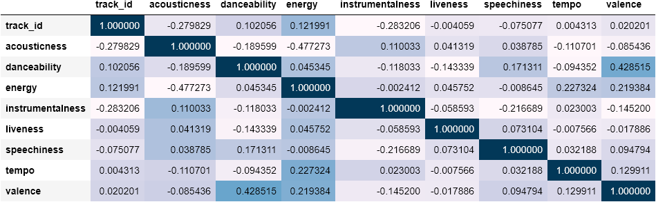
归一化特征数据 (Normalizing the feature data)
The output above does not show any significantly strong correlations. Hence we can proceed to reducing the number of features using ‘Principal Component Analysis’ (PCA).
上面的输出没有显示任何明显的强相关性。 因此,我们可以使用“主成分分析”(PCA)来减少特征数量。
The variance between genres can be explained by a few features. PCA rotates the data along the axis of highest variance, thus allowing us to determine the relative contribution of each feature of our data towards the variance between classes.
类型之间的差异可以通过一些功能来解释。 PCA沿最大方差轴旋转数据,从而使我们能够确定数据的每个特征对类之间方差的相对贡献。
However, PCA uses the absolute variance of a feature to rotate the data. This means that a feature with a broader range of values will overpower and bias the algorithm relative to the other features. To handle this, let us first normalize the data through standardization to generate all features with mean = 0 and standard deviation = 1 as seen below.
但是,PCA使用要素的绝对方差来旋转数据。 这意味着具有较宽值范围的功能将使其他算法无法胜任并且会使算法产生偏差。 为了解决这个问题,让我们首先通过标准化对数据进行归一化,以生成均值= 0和标准偏差= 1的所有特征,如下所示。
# Defining the features
features = echo_tracks.drop(columns=['genre_top', 'track_id'])

# Defining labels
labels = echo_tracks['genre_top']# Importing the StandardScaler
from sklearn.preprocessing import StandardScaler

# Scaling the features and setting the values to a new variable
scaler = StandardScaler()
scaled_train_features = scaler.fit_transform(features)
比例数据的主成分分析 (Principal Component Analysis on scaled data)
We are now ready to use PCA to determine by how much we can reduce the dimensionality of the data. Further, to find the number of components to use ahead, we can construct scree-plots and cumulative explained ratio plots. Scree-plots display the number of components against the variance explained by each component, sorted in descending order of variance. The ‘elbow’ that is a steep drop from one data point to the next, seen in the plot, decides an appropriate cut-off.
现在,我们准备使用PCA来确定我们可以减少多少数据维数。 此外,要找到预先要使用的组件数量,我们可以构建卵形图和累积解释比率图。 细目图显示了针对每个组件说明的方差的组件数,并按方差降序排列。 从图中可以看出,从一个数据点到另一个数据点的急剧下降的“弯头”决定了适当的截止点。
%matplotlib inline

# Importing the plotting module and PCA
import matplotlib.pyplot as plt
from sklearn.decomposition import PCA

# Getting explained variance ratios from PCA using all features
pca = PCA()
pca.fit(scaled_train_features)
exp_variance = pca.explained_variance_ratio_

# Plotting the explained variance using a barplot
fig, ax = plt.subplots()
ax.bar(range(pca.n_components_), exp_variance)
ax.set_xlabel('Principal Component #')Text(0.5, 0, 'Principal Component #')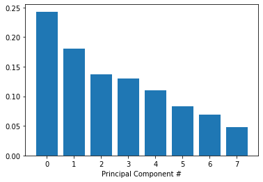
PCA的进一步可视化 (Further visualization of PCA)
The scree-plot above does not come up with a clear elbow so instead, let us look at the cumulative explained variance plot to determine how many features are required to explain, approximately 85% of the variance.
上面的卵石图没有清晰的弯头,因此,让我们看一下累积的解释方差图,以确定需要多少要素来解释,大约是方差的85%。
# Import numpy
import numpy as np

# Calculate the cumulative explained variance
cum_exp_variance = np.cumsum(exp_variance)

# Plot the cumulative explained variance and draw a dashed line at 0.85.
fig, ax = plt.subplots()
ax.plot(cum_exp_variance)
ax.axhline(y=0.85, linestyle='--')

# choose the n_components where about 85% of our variance can be explained
n_components = 6

# Perform PCA with the chosen number of components and project data onto components
pca = PCA(n_components, random_state=10)
pca.fit(scaled_train_features)
pca_projection =  pca.transform(scaled_train_features)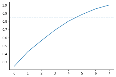
逻辑回归模型 (Logistic Regression Model)
Now we can use the lower dimensional PCA projection of the data to classify songs into genres. Let us build a logistic regression model by first splitting our dataset into ‘train’ and ‘test’ subsets, where the ‘train’ is used to train our model while the ‘test’ dataset allows for model performance validation. Further, Logistic Regression uses the logistic function to calculate the odds that a given data point belongs to a particular class.
现在,我们可以使用数据的低维PCA投影将歌曲分类为流派。 让我们通过首先将数据集分为“训练”和“测试”子集来构建逻辑回归模型,其中“训练”用于训练我们的模型,而“测试”数据集用于验证模型性能。 此外,逻辑回归使用逻辑函数来计算给定数据点属于特定类别的几率。
# Import train_test_split function
from sklearn.model_selection import train_test_split

# Split our data
train_features, test_features, train_labels, test_labels =  train_test_split(pca_projection, labels, random_state=10)# Import LogisticRegression
from sklearn.linear_model import LogisticRegression

# Training our logisitic regression
logreg = LogisticRegression(random_state=10)
logreg.fit(train_features, train_labels)
pred_labels_logit = logreg.predict(test_features)

# Creating the classification report for the model
from sklearn.metrics import classification_report
class_rep_log = classification_report(test_labels, pred_labels_logit)

print("Logistic Regression: \n", class_rep_log)Logistic Regression:
               precision    recall  f1-score   support

     Hip-Hop       0.77      0.54      0.64       235
        Rock       0.90      0.96      0.93       966

    accuracy                           0.88      1201
   macro avg       0.83      0.75      0.78      1201
weighted avg       0.87      0.88      0.87      1201
平衡数据以获得更好的性能 (Balancing the data for better performance)
The classification report shows us that rock songs are fairly well classified, but hip-hop songs are disproportionately misclassified as rock songs. There are far more data points for the rock classification than for hip-hop which skew our model’s ability to distinguish between classes. This also means that most of our logistic model’s accuracy is driven by its ability to classify just rock songs and these are hence not very good results.
分类报告显示,摇滚歌曲的分类相当不错,但嘻哈歌曲被错误地归类为摇滚歌曲。 岩石分类的数据要比街舞的数据点多,这使我们的模型区分类别的能力有所偏离。 这也意味着我们大多数逻辑模型的准确性受其仅对摇滚歌曲进行分类的能力所驱动,因此,这些结果并不是很好。
To account for this, we can weight the value of a correct classification in each class inversely to the occurrence of data points for each class.
为了解决这个问题,我们可以将每个类别中正确分类的值与每个类别中数据点的出现成反比。
# Subset a balanced proportion of data points
hop_only = echo_tracks.loc[echo_tracks['genre_top'] == 'Hip-Hop']
rock_only = echo_tracks.loc[echo_tracks['genre_top'] == 'Rock']

# subset only the rock songs, and take a sample the same size as there are hip-hop songs
rock_only = rock_only.sample(hop_only.shape[0], random_state=10)

# Concatenate the dataframes hop_only and rock_only
rock_hop_bal = pd.concat([rock_only, hop_only])

# The features, labels, and pca projection are created for the balanced dataframe
features = rock_hop_bal.drop(['genre_top', 'track_id'], axis=1)
labels = rock_hop_bal['genre_top']
pca_projection = pca.fit_transform(scaler.fit_transform(features))

# Redefine the train and test set with the pca_projection from the balanced data
train_features, test_features, train_labels, test_labels = train_test_split(
    pca_projection, labels, random_state=10)rock_hop_bal.info()<class 'pandas.core.frame.DataFrame'>
Int64Index: 1820 entries, 773 to 4801
Data columns (total 10 columns):
 #   Column            Non-Null Count  Dtype
---  ------            --------------  -----
 0   track_id          1820 non-null   int64
 1   acousticness      1820 non-null   float64
 2   danceability      1820 non-null   float64
 3   energy            1820 non-null   float64
 4   instrumentalness  1820 non-null   float64
 5   liveness          1820 non-null   float64
 6   speechiness       1820 non-null   float64
 7   tempo             1820 non-null   float64
 8   valence           1820 non-null   float64
 9   genre_top         1820 non-null   object
dtypes: float64(8), int64(1), object(1)
memory usage: 156.4+ KB
平衡会改善模型偏差吗? (Balancing improves model bias?)
The dataset is now balanced, but it has removed a lot of data points. Let us now test to see if balancing our data improves model bias towards the ‘Rock’ classification while retaining overall classification performance.
数据集现在已平衡,但已删除了许多数据点。 现在让我们测试一下,看看平衡数据是否可以改善模型对“ Rock”分类的偏见,同时又能保持整体分类性能。
# Training our logistic regression on the balanced data
logreg = LogisticRegression(random_state=10)
logreg.fit(train_features, train_labels)
pred_labels_logit = logreg.predict(test_features)
print("Logistic Regression: \n", classification_report(test_labels, pred_labels_logit))Logistic Regression:
               precision    recall  f1-score   support

     Hip-Hop       0.84      0.80      0.82       230
        Rock       0.80      0.85      0.83       225

    accuracy                           0.82       455
   macro avg       0.82      0.82      0.82       455
weighted avg       0.82      0.82      0.82       455
交叉验证评估 (Cross-validation for evaluation)
Balancing our data has removed bias but to get a good sense of actual performance, we can apply called cross-validation (CV). CV attempts to split the data multiple ways and test the model on each of the splits. Hereby, K-fold CV first splits the data into K different, equally sized subsets and iteratively uses each subset as a test set while using the remainder of the data as train sets. Finally, it aggregates the results from each fold and gives out a final model performance score.
平衡我们的数据可以消除偏差,但是为了获得良好的实际效果,我们可以应用称为交叉验证(CV)的方法。 CV尝试以多种方式拆分数据并在每个拆分中测试模型。 因此,K折CV首先将数据拆分为K个大小相同的不同子集,然后将每个子集迭代用作测试集,而将其余数据用作训练集。 最后,它汇总各折的结果,并给出最终的模型性能分数。
from sklearn.model_selection import KFold, cross_val_score

# Setting up K-fold cross-validation
kf = KFold(10)

logreg = LogisticRegression(random_state=10)

# Training our model using KFold cv
logit_score = cross_val_score(logreg, pca_projection, labels, cv=kf)

# Print the mean of each array o scores
print("Logistic Regression:", np.mean(logit_score))Logistic Regression: 0.782967032967033
翻译自: https://medium.com/analytics-vidhya/classify-song-genres-from-audio-data-a54107f95b34
原始音频数据合成音频文件
相关文章

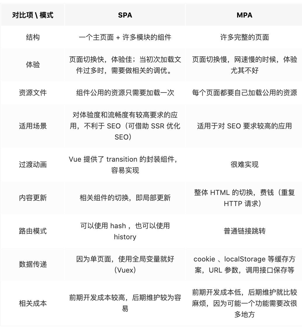
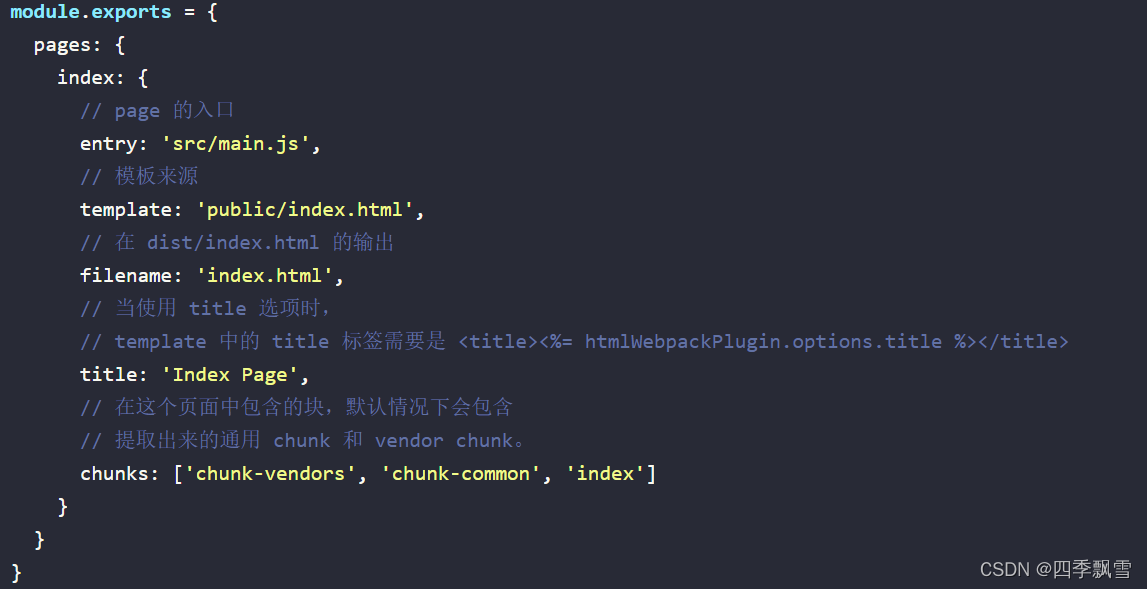
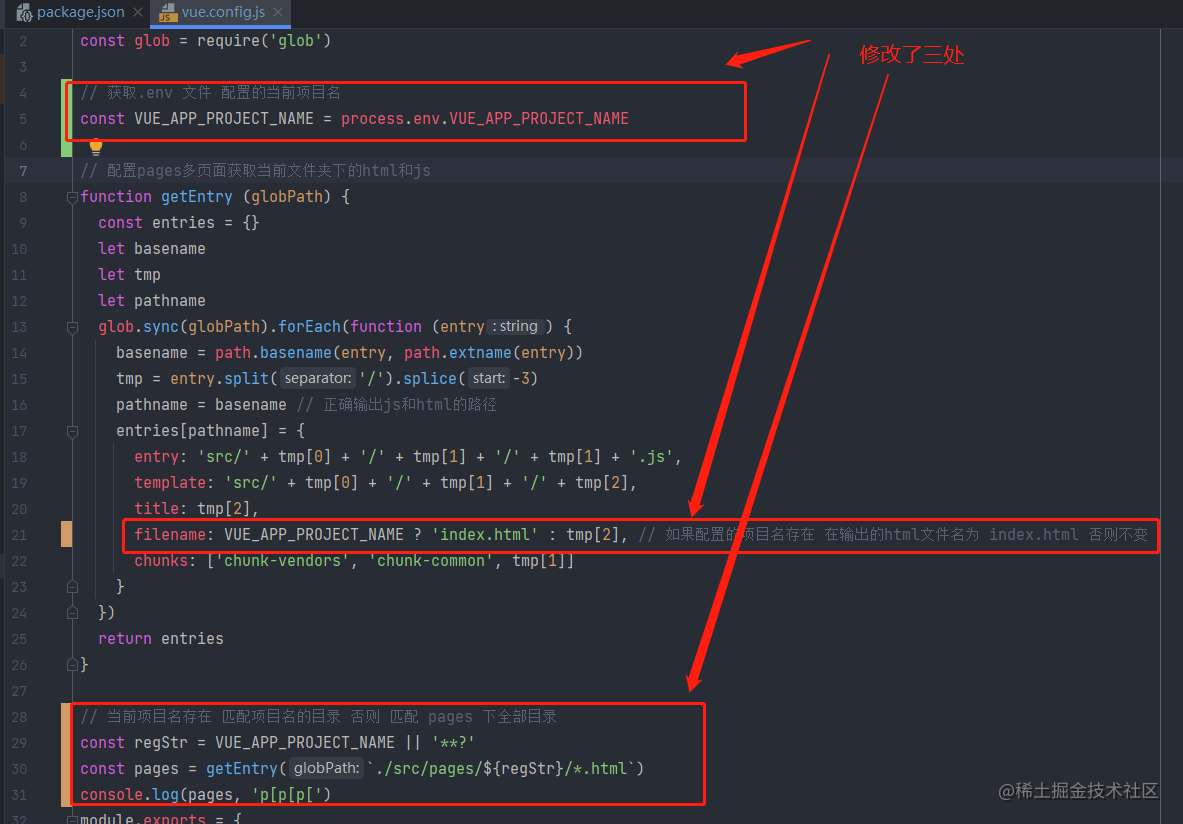
vue实现多页面应用

创建Vue单页面应用的3种方法
单页和多页应用(vue.js学习笔记)

Vue-router: 实现纯前端多页面应用(Vuecli+Element UI)

vue3+vite配置多页应用
51、Vue 单页面应用
vue多页面入口配置


nginx部署多个vue多页面项目
vue多页实践-开发

vue3搭建多页面应用的方法

vue实现多页面应用开发,包含项目之间跳转


vue配置多页面应用
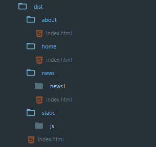
vue打包多个html,vue多页面应用打包配置
Vue多页面应用开发
