目录
前言
knn vs. svm
svm & linear classifier
bias trick
loss function
regularization
optimization
代码主体
导入数据及预处理
svm计算loss_function和梯度
验证梯度公式是否正确
比较运行时间
svm训练及预测,结果可视化
通过corss-validation来选定参数,结果可视化
具体实现
svm损失函数
训练与预测
通过数值分析检查梯度公式是否写正确
前言
knn vs. svm
之前是knn实现分类,其基本原理是定义一个distance metric,用这个metric衡量test instance到所有train set 中的instance的距离,结果就是loss objective。
这儿的svm实质上是一样的。只不过,svm做了两个小的改变。一是,svm通过train set,学习到了属于每个class的template(具体方法后面说),因此在predict的时候,test instance不再需要与所有的train data比较,只要与一个template比较,这个template就是后面要说到的W ,W是一个weight matrix,它的每一行就相当于一个template。行数等于定义的class 数量。二是svm通过Wx这样的矩阵点乘代替了knn的L1或L2 distance。
svm & linear classifier
svm属于linear classifier。linear classifier:,其中的W叫做weights,b叫做bias vector或者叫parameters interchangeably。
linear classifier可以理解为将一系列的data映射到classes上。以图像分类为例,图像的像素个数理解为维数,那么每个图片在就是在这个高维空间里的一个点。但高维是不能可视化的,为了理解,用二维草图做一个类比,用来理解线性分类器的作用。
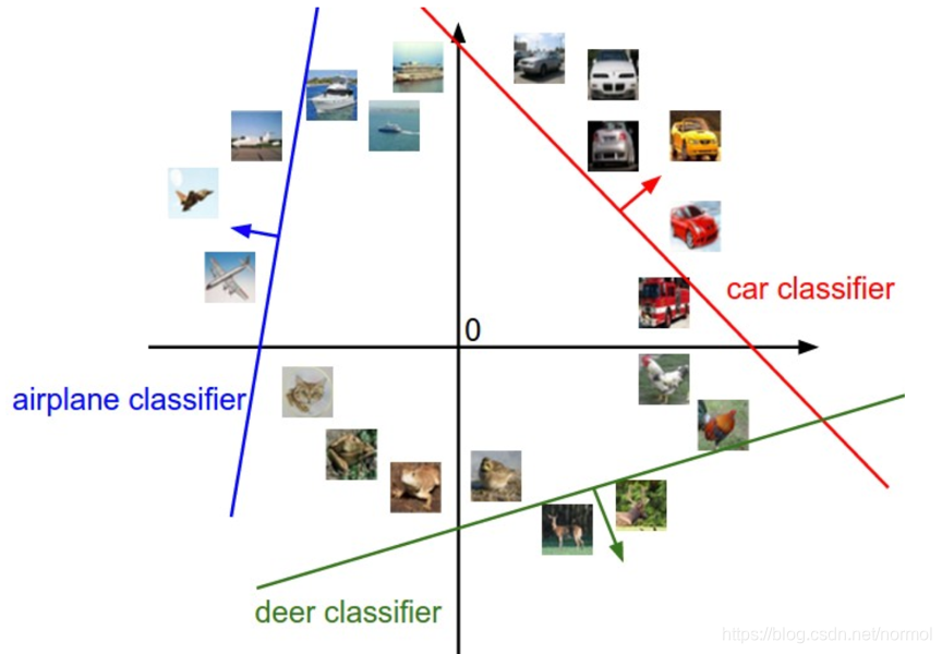
如上图所示,若图片恰好落在线上,证明其score等于0,离线越远,score的绝对值也就越大,箭头方向指向score的正增长方向。
bias trick
其中要解释下b,即bias。由线性公式或者图片可以知道,若没有b,那么所有的线都将经过原点,对于高维来说,就是只要W取全零,那么score一定得0,这显然是不对的,因此为了能使其偏移,就得加上b。在程序实现时,全都是矩阵操作,为了能统一,我们会对data进行预处理,即append 一个1,这样就可以以一个矩阵乘法实现Wx+b的操作,如下图所示。

loss function
wx+b的结果就是我们的outcome了,光有outcome显然没有用,在knn中,我们通过选取k 个outcome最高的nearest neighbors来vote出结果,这儿我们需要定义一个loss function,来衡量wx+b的结果与我们真正想要的结果相差多少。或者说这个结果损失了多少信息。
解释一下公式的含义,首先上述的x都是append 1之后的结果,因此不需要+b。
j代表第j个class,i代表第i个样品。计算的例子可以看这篇文章svm 损失函数以及其梯度推导,这儿在直观上理解一下,不考虑delta的话,就是对于一个样品而言,其预测出来的结果是一个score vector,每个元算的含义是这个样品在每个j-th class的得分。那么如果这个样品的真正分类是“car”,且这个分类器给出的这个样品在car上的得分是10,如果其余类别的得分低于10,根据max函数(常被叫做 hinge loss),损失为0,但如果在“cat”上的得分为12,自然就不对了,于是max会得量化差距为多少。delta在这儿的作用就是边界,我们预设定的参数,希望正确分类的分数与其他的分数相差多少,如下图所示

其实这个delta的取值对结果并没有影响,一般而言取1,原因在下面的regularization会说。
regularization
之所以需要这一步,是因为上面的loss function是有问题的。
比如,我们有一个分类器正确的进行了所有的分类,那么我们的L为0,但是,对W乘以任何常数,结果仍不会改变。
这样会有问题,例如W衡量出的关于某个样品cat种类得分为30,真正类别的得分为15,他们的差值为15,但若W变为2W,那么差值就变成了30.
于是我们提出了regularization function 。注意,这个不是关于输入data的函数,而是关于weights的。加上它的之后,不仅修复了之前提到的bug,还使得我们的模型更加general,例如,对于输入数据x=[1,1,1,1], w1=[0.25,0.25,0.25,0.25], w2=[1,0,0,0],虽然两个乘积结果一样,但w1的regularization loss要小于w2。根据公示可以知道,其更倾向于选择weight更小,更分散的。对应于实际,就是说不会在某一个像素上有很大的weight,而是比重更加均匀。这也避免的overfitting。
最后我们的loss function变成了:
setting Delta and lambda
上一个小节提到,delta的选取并不重要,就是因为有lambda缩放regualarization loss,这两个参数实质上做了相同的tradeoff。
若我们选择很大的margin,也就是delta很大,但我们的lambda则可以选的很小,因此上面说,delta的取值并不重要。
optimization
有了上述的评定标准,我们就可以选择w了,选择w的过程就是使loss function最小的过程。
具体是通过梯度实现的,这儿不再详述,可参考svm 损失函数以及其梯度推导
代码主体
导入数据及预处理
# Run some setup code for this notebook.
"""
进行一些设置
"""import random
import numpy as np
from cs231n.data_utils import load_CIFAR10
import matplotlib.pyplot as pltfrom __future__ import print_function# This is a bit of magic to make matplotlib figures appear inline in the
# notebook rather than in a new window.
%matplotlib inline
plt.rcParams['figure.figsize'] = (10.0, 8.0) # set default size of plots
plt.rcParams['image.interpolation'] = 'nearest'
plt.rcParams['image.cmap'] = 'gray'# Some more magic so that the notebook will reload external python modules;
# see http://stackoverflow.com/questions/1907993/autoreload-of-modules-in-ipython
%load_ext autoreload
%autoreload 2# Load the raw CIFAR-10 data.
cifar10_dir = 'cs231n/datasets/cifar-10-batches-py'# Cleaning up variables to prevent loading data multiple times (which may cause memory issue)
try:del X_train, y_traindel X_test, y_testprint('Clear previously loaded data.')
except:passX_train, y_train, X_test, y_test = load_CIFAR10(cifar10_dir)# As a sanity check, we print out the size of the training and test data.
print('Training data shape: ', X_train.shape)
print('Training labels shape: ', y_train.shape)
print('Test data shape: ', X_test.shape)
print('Test labels shape: ', y_test.shape)# Visualize some examples from the dataset.
# We show a few examples of training images from each class.
classes = ['plane', 'car', 'bird', 'cat', 'deer', 'dog', 'frog', 'horse', 'ship', 'truck']
num_classes = len(classes)
samples_per_class = 7
for y, cls in enumerate(classes):idxs = np.flatnonzero(y_train == y)idxs = np.random.choice(idxs, samples_per_class, replace=False)for i, idx in enumerate(idxs):plt_idx = i * num_classes + y + 1plt.subplot(samples_per_class, num_classes, plt_idx)plt.imshow(X_train[idx].astype('uint8'))plt.axis('off')if i == 0:plt.title(cls)
plt.show()# Split the data into train, val, and test sets. In addition we will
# create a small development set as a subset of the training data;
# we can use this for development so our code runs faster.
num_training = 49000
num_validation = 1000
num_test = 1000
num_dev = 500# Our validation set will be num_validation points from the original
# training set.
mask = range(num_training, num_training + num_validation)
X_val = X_train[mask]
y_val = y_train[mask]# Our training set will be the first num_train points from the original
# training set.
mask = range(num_training)
X_train = X_train[mask]
y_train = y_train[mask]# We will also make a development set, which is a small subset of
# the training set.
mask = np.random.choice(num_training, num_dev, replace=False)
X_dev = X_train[mask]
y_dev = y_train[mask]# We use the first num_test points of the original test set as our
# test set.
mask = range(num_test)
X_test = X_test[mask]
y_test = y_test[mask]print('Train data shape: ', X_train.shape)
print('Train labels shape: ', y_train.shape)
print('Validation data shape: ', X_val.shape)
print('Validation labels shape: ', y_val.shape)
print('Test data shape: ', X_test.shape)
print('Test labels shape: ', y_test.shape)# Preprocessing: reshape the image data into rows
# or we could use X_train.reshape(row,col)
X_train = np.reshape(X_train, (X_train.shape[0], -1))
X_val = np.reshape(X_val, (X_val.shape[0], -1))
X_test = np.reshape(X_test, (X_test.shape[0], -1))
X_dev = np.reshape(X_dev, (X_dev.shape[0], -1))# As a sanity check, print out the shapes of the data
print('Training data shape: ', X_train.shape)
print('Validation data shape: ', X_val.shape)
print('Test data shape: ', X_test.shape)
print('dev data shape: ', X_dev.shape)# second: subtract the mean image from train and test data
#https://tomaszkacmajor.pl/index.php/2016/04/24/data-preprocessing/
X_train -= mean_image
X_val -= mean_image
X_test -= mean_image
X_dev -= mean_image# third: append the bias dimension of ones (i.e. bias trick) so that our SVM
# only has to worry about optimizing a single weight matrix W.
X_train = np.hstack([X_train, np.ones((X_train.shape[0], 1))])
X_val = np.hstack([X_val, np.ones((X_val.shape[0], 1))])
X_test = np.hstack([X_test, np.ones((X_test.shape[0], 1))])
X_dev = np.hstack([X_dev, np.ones((X_dev.shape[0], 1))])print(X_train.shape, X_val.shape, X_test.shape, X_dev.shape)
svm计算loss_function和梯度
# Evaluate the naive implementation of the loss we provided for you:
from cs231n.classifiers.linear_svm import svm_loss_naive
import time# generate a random SVM weight matrix of small numbers
W = np.random.randn(3073, 10) * 0.0001 loss, grad = svm_loss_naive(W, X_dev, y_dev, 0.000005)
print('loss: %f' % (loss, ))# Once you've implemented the gradient, recompute it with the code below
# and gradient check it with the function we provided for you# Compute the loss and its gradient at W.
loss, grad = svm_loss_naive(W, X_dev, y_dev, 0.0)
验证梯度公式是否正确
# Numerically compute the gradient along several randomly chosen dimensions, and
# compare them with your analytically computed gradient. The numbers should match
# almost exactly along all dimensions.
from cs231n.gradient_check import grad_check_sparse
f = lambda w: svm_loss_naive(w, X_dev, y_dev, 0.0)[0]
grad_numerical = grad_check_sparse(f, W, grad)# do the gradient check once again with regularization turned on
# you didn't forget the regularization gradient did you?
loss, grad = svm_loss_naive(W, X_dev, y_dev, 5e1)
f = lambda w: svm_loss_naive(w, X_dev, y_dev, 5e1)[0]
grad_numerical = grad_check_sparse(f, W, grad)
比较运行时间
# Next implement the function svm_loss_vectorized; for now only compute the loss;
# we will implement the gradient in a moment.
tic = time.time()
loss_naive, grad_naive = svm_loss_naive(W, X_dev, y_dev, 0.000005)
toc = time.time()
print('Naive loss: %e computed in %fs' % (loss_naive, toc - tic))from cs231n.classifiers.linear_svm import svm_loss_vectorized
tic = time.time()
loss_vectorized, _ = svm_loss_vectorized(W, X_dev, y_dev, 0.000005)
toc = time.time()
print('Vectorized loss: %e computed in %fs' % (loss_vectorized, toc - tic))# The losses should match but your vectorized implementation should be much faster.
print('difference: %f' % (loss_naive - loss_vectorized))# Complete the implementation of svm_loss_vectorized, and compute the gradient
# of the loss function in a vectorized way.# The naive implementation and the vectorized implementation should match, but
# the vectorized version should still be much faster.
tic = time.time()
_, grad_naive = svm_loss_naive(W, X_dev, y_dev, 0.000005)
toc = time.time()
print('Naive loss and gradient: computed in %fs' % (toc - tic))tic = time.time()
_, grad_vectorized = svm_loss_vectorized(W, X_dev, y_dev, 0.000005)
toc = time.time()
print('Vectorized loss and gradient: computed in %fs' % (toc - tic))# The loss is a single number, so it is easy to compare the values computed
# by the two implementations. The gradient on the other hand is a matrix, so
# we use the Frobenius norm to compare them.
difference = np.linalg.norm(grad_naive - grad_vectorized, ord='fro')
print('difference: %f' % difference)
svm训练及预测,结果可视化
# In the file linear_classifier.py, implement SGD in the function
# LinearClassifier.train() and then run it with the code below.
from cs231n.classifiers import LinearSVM
svm = LinearSVM()
tic = time.time()
loss_hist = svm.train(X_train, y_train, learning_rate=1e-7, reg=2.5e4,num_iters=1500, verbose=True)
toc = time.time()
print('That took %fs' % (toc - tic))# A useful debugging strategy is to plot the loss as a function of
# iteration number:
plt.plot(loss_hist)
plt.xlabel('Iteration number')
plt.ylabel('Loss value')
plt.show()# Write the LinearSVM.predict function and evaluate the performance on both the
# training and validation set
y_train_pred = svm.predict(X_train)
print('training accuracy: %f' % (np.mean(y_train == y_train_pred), ))
y_val_pred = svm.predict(X_val)
print('validation accuracy: %f' % (np.mean(y_val == y_val_pred), ))
通过corss-validation来选定参数,结果可视化
# Use the validation set to tune hyperparameters (regularization strength and
# learning rate). You should experiment with different ranges for the learning
# rates and regularization strengths; if you are careful you should be able to
# get a classification accuracy of about 0.4 on the validation set.
learning_rates = [1e-7, 5e-5]
regularization_strengths = [1.5e4, 5e4]# results is dictionary mapping tuples of the form
# (learning_rate, regularization_strength) to tuples of the form
# (training_accuracy, validation_accuracy). The accuracy is simply the fraction
# of data points that are correctly classified.
results = {}
best_val = -1   # The highest validation accuracy that we have seen so far.
best_svm = None # The LinearSVM object that achieved the highest validation rate.################################################################################
# TODO:                                                                        #
# Write code that chooses the best hyperparameters by tuning on the validation #
# set. For each combination of hyperparameters, train a linear SVM on the      #
# training set, compute its accuracy on the training and validation sets, and  #
# store these numbers in the results dictionary. In addition, store the best   #
# validation accuracy in best_val and the LinearSVM object that achieves this  #
# accuracy in best_svm.                                                        #
#                                                                              #
# Hint: You should use a small value for num_iters as you develop your         #
# validation code so that the SVMs don't take much time to train; once you are #
# confident that your validation code works, you should rerun the validation   #
# code with a larger value for num_iters.                                      #
################################################################################range_lr = np.linspace(learning_rates[0],learning_rates[1],3)
range_reg = np.linspace(regularization_strengths[0],regularization_strengths[1],3)for cur_lr in range_lr: #go over the learning ratesfor cur_reg in range_reg:#go over the regularization strengthsvm = LinearSVM()svm.train(X_train, y_train, learning_rate=cur_lr, reg=cur_reg,num_iters=1500, verbose=False)y_train_pred = svm.predict(X_train)train_acc = np.mean(y_train == y_train_pred)y_val_pred = svm.predict(X_val)val_acc = np.mean(y_val == y_val_pred)# FIX storing resultsresults[(cur_lr,cur_reg)] = (train_acc,val_acc)if val_acc > best_val:best_val = val_accbest_svm = svm################################################################################
#                              END OF YOUR CODE                                #
################################################################################# Print out results.for lr, reg in sorted(results):train_accuracy, val_accuracy = results[(lr, reg)]print('lr %e reg %e train accuracy: %f val accuracy: %f' % (lr, reg, train_accuracy, val_accuracy))print('best validation accuracy achieved during cross-validation: %f' % best_val)# Visualize the cross-validation results
import math
x_scatter = [math.log10(x[0]) for x in results]
y_scatter = [math.log10(x[1]) for x in results]# plot training accuracy
marker_size = 100
colors = [results[x][0] for x in results]
plt.subplot(2, 1, 1)
plt.scatter(x_scatter, y_scatter, marker_size, c=colors)
plt.colorbar()
plt.xlabel('log learning rate')
plt.ylabel('log regularization strength')
plt.title('CIFAR-10 training accuracy')# plot validation accuracy
colors = [results[x][1] for x in results] # default size of markers is 20
plt.subplot(2, 1, 2)
plt.scatter(x_scatter, y_scatter, marker_size, c=colors)
plt.colorbar()
plt.xlabel('log learning rate')
plt.ylabel('log regularization strength')
plt.title('CIFAR-10 validation accuracy')
plt.show()# Evaluate the best svm on test set
y_test_pred = best_svm.predict(X_test)
test_accuracy = np.mean(y_test == y_test_pred)
print('linear SVM on raw pixels final test set accuracy: %f' % test_accuracy)# Visualize the learned weights for each class.
# Depending on your choice of learning rate and regularization strength, these may
# or may not be nice to look at.
w = best_svm.W[:-1,:] # strip out the bias
w = w.reshape(32, 32, 3, 10)
w_min, w_max = np.min(w), np.max(w)
classes = ['plane', 'car', 'bird', 'cat', 'deer', 'dog', 'frog', 'horse', 'ship', 'truck']
for i in range(10):plt.subplot(2, 5, i + 1)# Rescale the weights to be between 0 and 255wimg = 255.0 * (w[:, :, :, i].squeeze() - w_min) / (w_max - w_min)plt.imshow(wimg.astype('uint8'))plt.axis('off')plt.title(classes[i])
具体实现
svm损失函数
方式一
import numpy as np
from random import shuffledef svm_loss_naive(W, X, y, reg):"""Structured SVM loss function, naive implementation (with loops).Inputs have dimension D, there are C classes, and we operate on minibatchesof N examples.Inputs:- W: A numpy array of shape (D, C) containing weights.- X: A numpy array of shape (N, D) containing a minibatch of data.- y: A numpy array of shape (N,) containing training labels; y[i] = c meansthat X[i] has label c, where 0 <= c < C.- reg: (float) regularization strengthReturns a tuple of:- loss as single float- gradient with respect to weights W; an array of same shape as W"""# Initialize loss and the gradient of W to zero.dW = np.zeros(W.shape)loss = 0.0num_classes = W.shape[1]num_train = X.shape[0]# Compute the data loss and the gradient.for i in range(num_train):  # For each image in training.scores = X[i].dot(W)correct_class_score = scores[y[i]]num_classes_greater_margin = 0for j in range(num_classes):  # For each calculated class score for this image.# Skip if images target class, no loss computed for that case.if j == y[i]:continue# Calculate our margin, delta = 1margin = scores[j] - correct_class_score + 1# Only calculate loss and gradient if margin condition is violated.if margin > 0:num_classes_greater_margin += 1# Gradient for non correct class weight.dW[:, j] = dW[:, j] + X[i, :]loss += margin# Gradient for correct class weight.dW[:, y[i]] = dW[:, y[i]] - X[i, :]*num_classes_greater_margin# Average our data loss across the batch.loss /= num_train# Add regularization loss to the data loss.loss += reg * np.sum(W * W)# Average our gradient across the batch and add gradient of regularization term.dW = dW /num_train + 2*reg *Wreturn loss, dW
方式二
import numpy as np
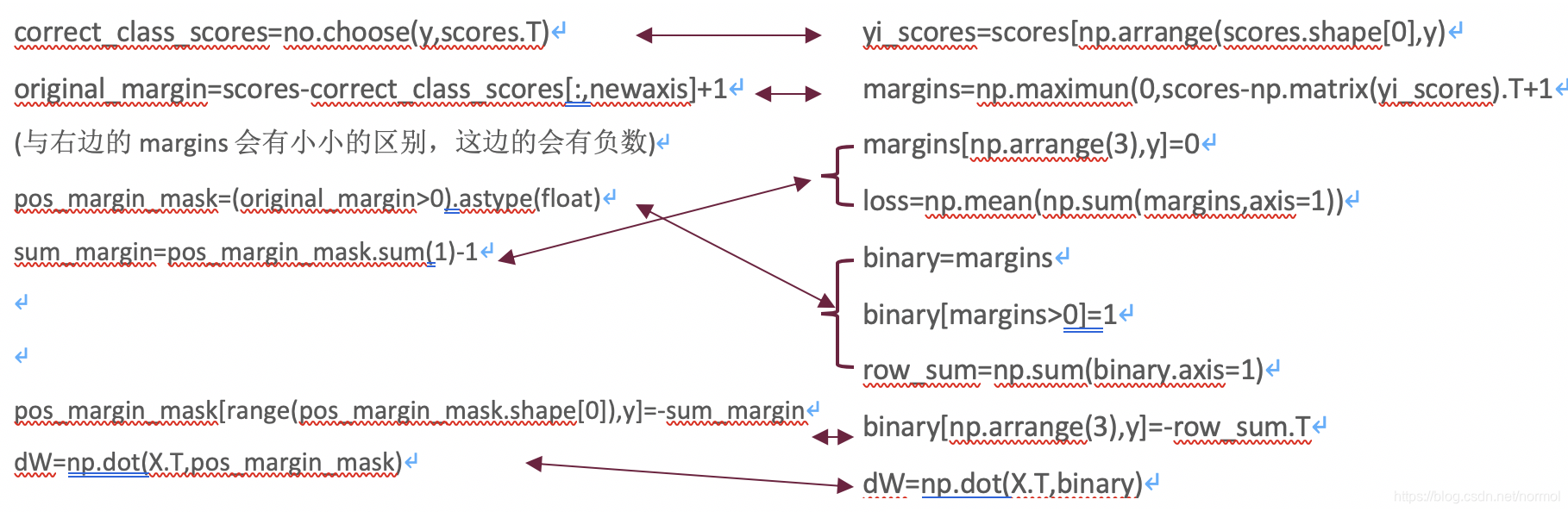
from random import shuffledef svm_loss_vectorized(W, X, y, reg):"""Structured SVM loss function, vectorized implementation.Inputs and outputs are the same as svm_loss_naive."""loss = 0.0dW = np.zeros(W.shape) # initialize the gradient as zero############################################################################## TODO: ## Implement a vectorized version of the structured SVM loss, storing the ## result in loss. ##############################################################################num_train = X.shape[0]scores = np.dot(X, W)"""除了可以用于list,choose还可以用于np.array类型。在机器学习中,通常a每行为一个sample,列数代表不同的feature。index中保存每个sample需要选出 feature的序号。那么可以通过以下操作在a中选出所有sample的目标feature:a = np.array([[1,2,3],[4,5,6],[7,8,9],[10,11,12]])index = np.array([0,2,1,0])np.choose(index,a.T)array([ 1, 6, 8, 10])"""correct_class_scores = np.choose(y, scores.T) # np.choose uses y to select elements from scores.T# Need to remove correct class scores as we dont calculate loss/margin for those.mask = np.ones(scores.shape, dtype=bool)mask[range(scores.shape[0]), y] = Falsescores_ = scores[mask].reshape(scores.shape[0], scores.shape[1]-1)# Calculate our margins all at once.margin = scores_ - correct_class_scores[..., np.newaxis] + 1# Only add margin to our loss if it's greater than 0, let's make# negative margins =0 so they dont change our loss.margin[margin < 0] = 0# Average our data loss over the size of batch and add reg. term to the loss.loss = np.sum(margin) / num_trainloss += reg * np.sum(W * W)############################################################################## END OF YOUR CODE ############################################################################################################################################################ TODO: ## Implement a vectorized version of the gradient for the structured SVM ## loss, storing the result in dW. ## ## Hint: Instead of computing the gradient from scratch, it may be easier ## to reuse some of the intermediate values that you used to compute the ## loss. ##############################################################################original_margin = scores - correct_class_scores[...,np.newaxis] + 1# Mask to identiy where the margin is greater than 0 (all we care about for gradient).pos_margin_mask = (original_margin > 0).astype(float)# Count how many times >0 for each image but dont count correct class hence -1sum_margin = pos_margin_mask.sum(1) - 1# Make the correct class margin be negative total of how many > 0pos_margin_mask[range(pos_margin_mask.shape[0]), y] = -sum_margin# Now calculate our gradient.dW = np.dot(X.T, pos_margin_mask)# Average over batch and add regularisation derivative.dW = dW / num_train + 2 * reg * W############################################################################## END OF YOUR CODE ##############################################################################return loss, dW前一篇文章也有vectorized implement,二者在理论上是一致的,下面的图是二者实现代码的比较
训练与预测
from __future__ import print_functionimport numpy as np
from cs231n.classifiers.linear_svm import *class LinearClassifier(object):def __init__(self):self.W = Nonedef train(self, X, y, learning_rate=1e-3, reg=1e-5, num_iters=100,batch_size=200, verbose=False):"""Train this linear classifier using stochastic gradient descent.Inputs:- X: A numpy array of shape (N, D) containing training data; there are Ntraining samples each of dimension D.- y: A numpy array of shape (N,) containing training labels; y[i] = cmeans that X[i] has label 0 <= c < C for C classes.- learning_rate: (float) learning rate for optimization.- reg: (float) regularization strength.- num_iters: (integer) number of steps to take when optimizing- batch_size: (integer) number of training examples to use at each step.- verbose: (boolean) If true, print progress during optimization.Outputs:A list containing the value of the loss function at each training iteration."""num_train, dim = X.shapenum_classes = np.max(y) + 1 # assume y takes values 0...K-1 where K is number of classesif self.W is None:# lazily initialize Wself.W = 0.001 * np.random.randn(dim, num_classes)# list of integers between 0 and length of X (these are our indicesX_indices = np.arange(num_train)# Run stochastic gradient descent to optimize Wloss_history = []for it in range(num_iters):X_batch = Noney_batch = None########################################################################## TODO:                                                                 ## Sample batch_size elements from the training data and their           ## corresponding labels to use in this round of gradient descent.        ## Store the data in X_batch and their corresponding labels in           ## y_batch; after sampling X_batch should have shape (dim, batch_size)   ## and y_batch should have shape (batch_size,)                           ##                                                                       ## Hint: Use np.random.choice to generate indices. Sampling with         ## replacement is faster than sampling without replacement.              ########################################################################### Choose 'batch_size' random values from X_indices.batch_indices = np.random.choice(X_indices,batch_size)# Get our batch from these indices.X_batch = X[batch_indices]y_batch = y[batch_indices]##########################################################################                       END OF YOUR CODE                                ########################################################################### evaluate loss and gradientloss, grad = self.loss(X_batch, y_batch, reg)loss_history.append(loss)# perform parameter update########################################################################## TODO:                                                                 ## Update the weights using the gradient and the learning rate.          ########################################################################### Gradient descent basic rule is just: weights += -(learning_rate * dW).self.W += -(learning_rate * grad)##########################################################################                       END OF YOUR CODE                                ##########################################################################if verbose and it % 100 == 0:print('iteration %d / %d: loss %f' % (it, num_iters, loss))return loss_historydef predict(self, X):"""Use the trained weights of this linear classifier to predict labels fordata points.Inputs:- X: A numpy array of shape (N, D) containing training data; there are Ntraining samples each of dimension D.Returns:- y_pred: Predicted labels for the data in X. y_pred is a 1-dimensionalarray of length N, and each element is an integer giving the predictedclass."""y_pred = np.zeros(X.shape[0])############################################################################ TODO:                                                                   ## Implement this method. Store the predicted labels in y_pred.            ############################################################################pred_scores = np.dot(X,self.W)y_pred = np.argmax(pred_scores, axis=1)############################################################################                           END OF YOUR CODE                              ############################################################################return y_preddef loss(self, X_batch, y_batch, reg):"""Compute the loss function and its derivative. Subclasses will override this.Inputs:- X_batch: A numpy array of shape (N, D) containing a minibatch of Ndata points; each point has dimension D.- y_batch: A numpy array of shape (N,) containing labels for the minibatch.- reg: (float) regularization strength.Returns: A tuple containing:- loss as a single float- gradient with respect to self.W; an array of the same shape as W"""passclass LinearSVM(LinearClassifier):""" A subclass that uses the Multiclass SVM loss function """def loss(self, X_batch, y_batch, reg):return svm_loss_vectorized(self.W, X_batch, y_batch, reg)
通过数值分析检查梯度公式是否写正确
from __future__ import print_function
def grad_check_sparse(f, x, analytic_grad, num_checks=10, h=1e-5):"""sample a few random elements and only return numericalin this dimensions."""for i in range(num_checks):ix = tuple([randrange(m) for m in x.shape])oldval = x[ix]x[ix] = oldval + h # increment by hfxph = f(x) # evaluate f(x + h)x[ix] = oldval - h # increment by hfxmh = f(x) # evaluate f(x - h)x[ix] = oldval # resetgrad_numerical = (fxph - fxmh) / (2 * h)grad_analytic = analytic_grad[ix]rel_error = abs(grad_numerical - grad_analytic) / (abs(grad_numerical) + abs(grad_analytic))print('numerical: %f analytic: %f, relative error: %e' % (grad_numerical, grad_analytic, rel_error))
import numpy as np
from random import randrange
ss