MATLAB | 有关数值矩阵、颜色图及颜色列表的技巧整理

这是一篇有关数值矩阵、颜色矩阵、颜色列表的技巧整合，会以随笔的形式想到哪写到哪，可能思绪会比较飘逸请大家见谅，本文大体分为以下几个部分：

数值矩阵用颜色显示
从颜色矩阵提取颜色
从颜色矩阵中提取数据
颜色列表相关函数
颜色测试图表的识别

数值矩阵用颜色显示

heatmap

我们最常用的肯定就是heatmap函数显示数值矩阵：

X=rand(10);
heatmap(X);

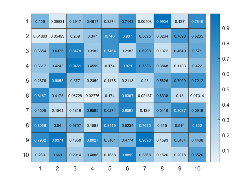
字体颜色可设置为透明：

X=rand(10);
HM=heatmap(X);
HM.CellLabelColor='none';

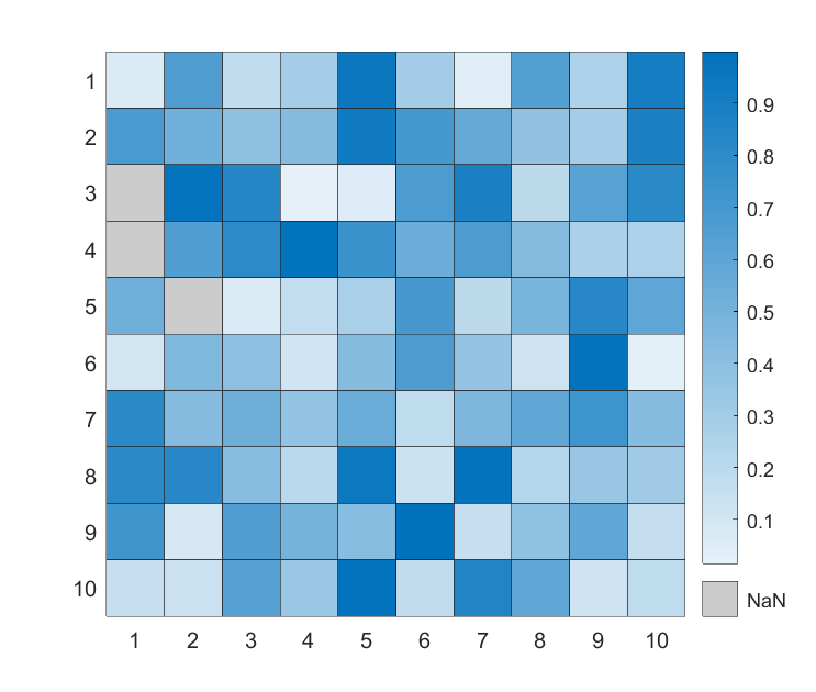
如果由NaN值，会显示为黑色：

X=rand(10);
X([3,4,15])=nan;
HM=heatmap(X);
HM.CellLabelColor='none';

这个颜色也可以改，比如改成浅灰色：

X=rand(10);
X([3,4,15])=nan;
HM=heatmap(X);
HM.CellLabelColor='none';
HM.MissingDataColor=[.8,.8,.8];

imagesc

imagesc随便加个colorbar就和heatmap非常像了，而且比较容易进行图像组合(heatmap的父类不能是axes)，但是没有边缘：

X=rand(10);
imagesc(X)
colormap(winter)
colorbar

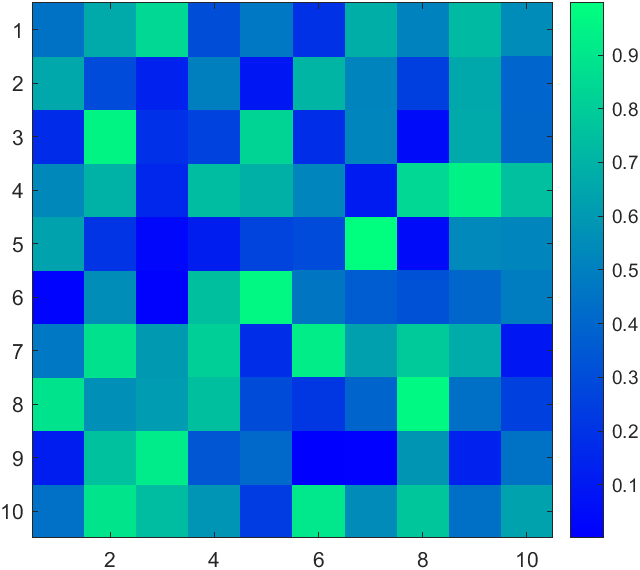
比较烦的是imagesc即使数据有NaN也会对其进行插值显示，好坏参半吧。

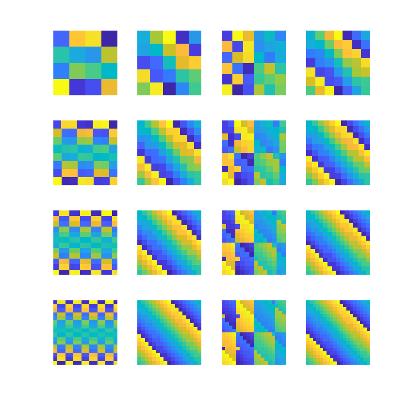
另外随便写了点代码发现MATLAB自带的幻方绘制挺有规律的hiahiahia:

for i=1:16ax=subplot(4,4,i);hold on;axis tight off equalX=magic(3+i);imagesc(X);
end

image

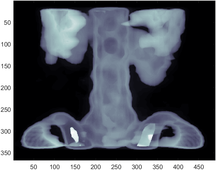
image函数单通道时也可以设置colormap来进行颜色映射：

load spine
image(X)
colormap(map)

pcolor

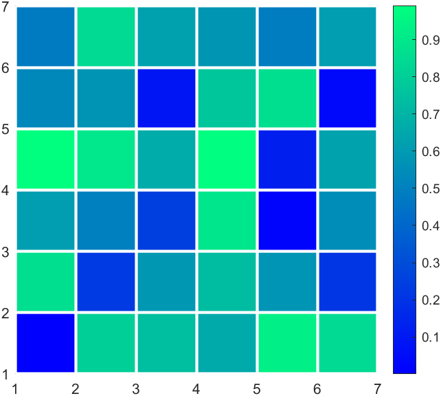
pcolor由于每个方块颜色都会使用左上角的数值来计算，因此会缺一行一列，我们可以补上一行一列nan:

X=rand(6);
X(end+1,:)=nan;
X(:,end+1)=nan;
pcolor(X);
colormap(winter)
colorbar

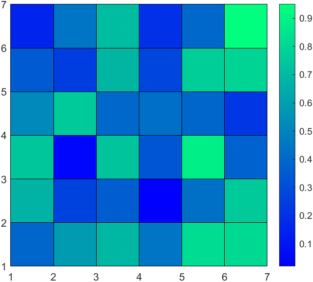
可修饰的东西就比较丰富了，比如边缘颜色：

X=rand(6);
X(end+1,:)=nan;
X(:,end+1)=nan;
pHdl=pcolor(X);
pHdl.EdgeColor=[1,1,1];
pHdl.LineWidth=2;
colormap(winter)
colorbar

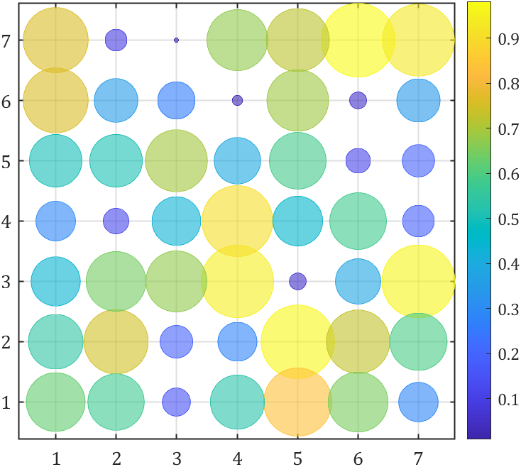
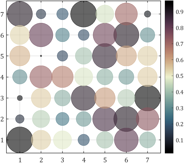
气泡图

气泡图大概也能冒充一下热图：

Z=rand(7);
[X,Y]=meshgrid(1:size(Z,2),1:size(Z,1));bubblechart(X(:),Y(:),Z(:),Z(:),'MarkerFaceAlpha',.6) 
colormap(parula)
colorbar
set(gca,'XTick',1:size(Z,2),'YTick',1:size(Z,1),'LineWidth',1,...'XGrid','on','YGrid','on','FontName','Cambria','FontSize',13)

随便写着玩

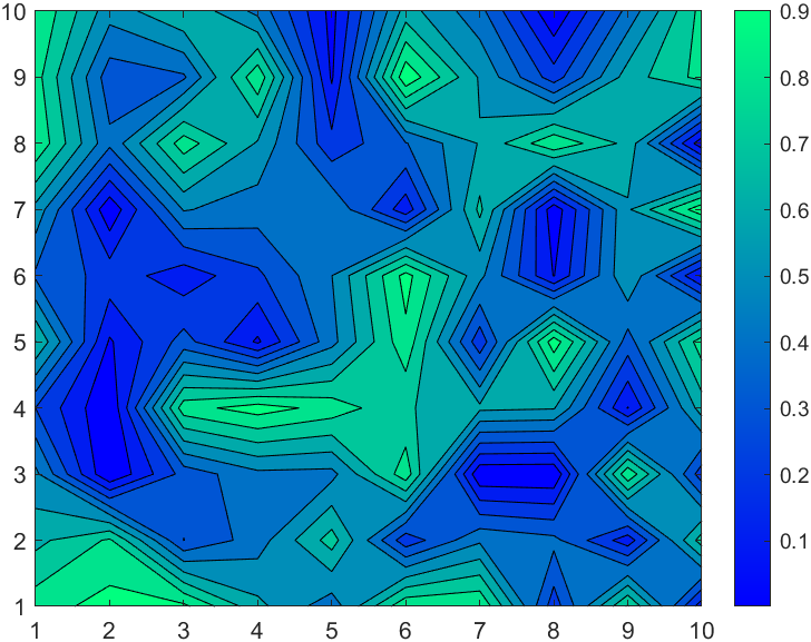
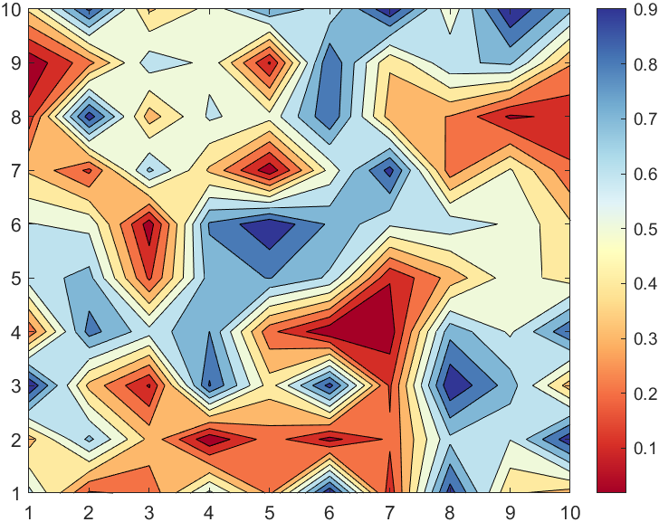
虽然surf函数调整视角也像是热图的样子，但是不打算讲了，反而等高线填充图虽然不像热图但是很有意思，感觉可以当作colormap展示的示例图：

X=rand(10);
CF=contourf(X);
colormap(winter)
colorbar

从颜色矩阵提取颜色

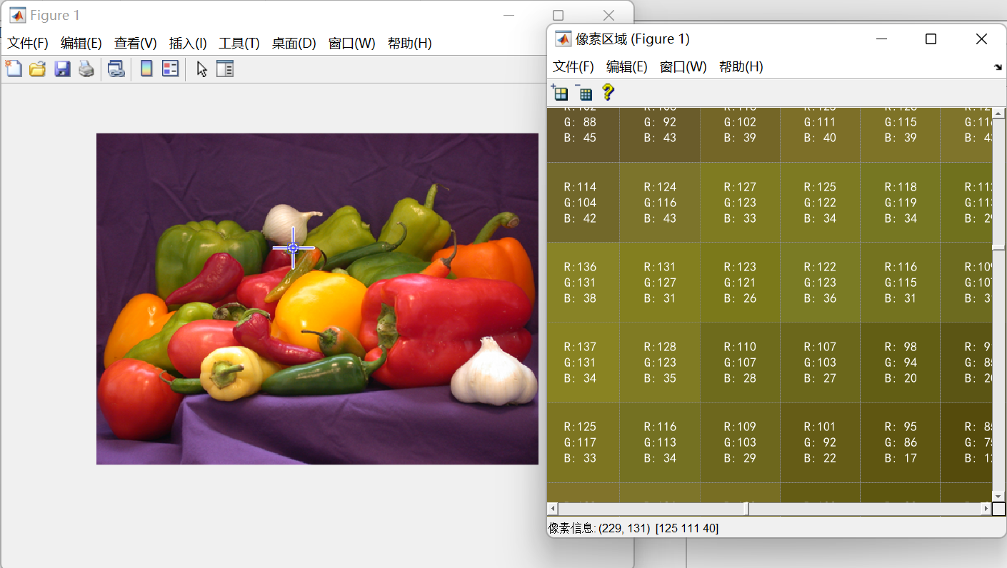
像素提取器

需要安装：
Image Processing Toolbox
图像处理工具箱.

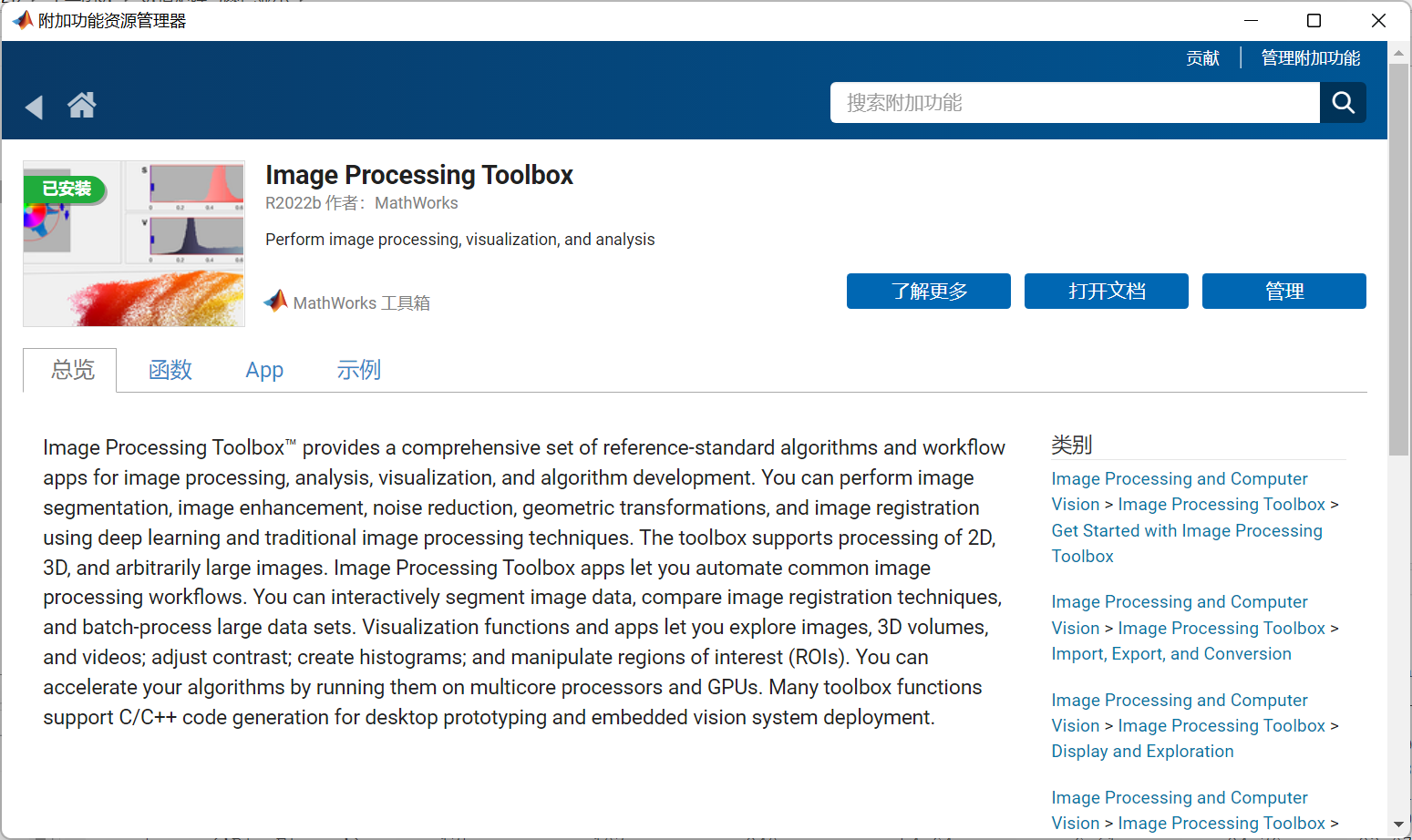
使用以下代码可以显示每个像素RGB值：

imshow('peppers.png')
impixelregion

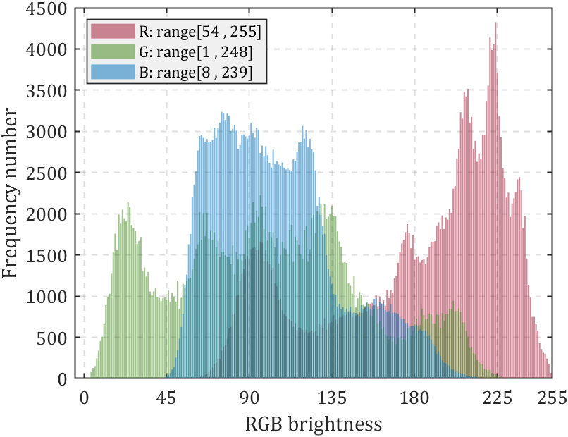
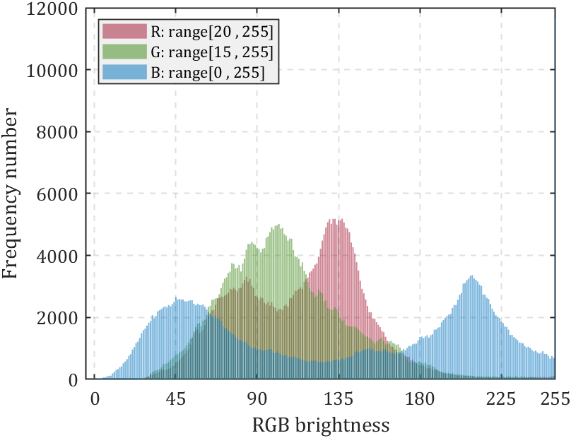
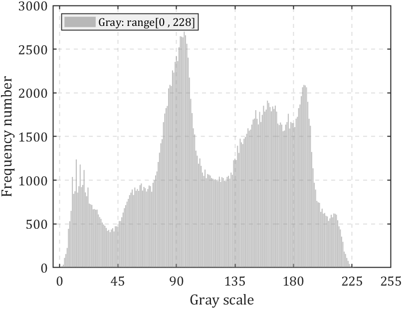
图片颜色统计小函数

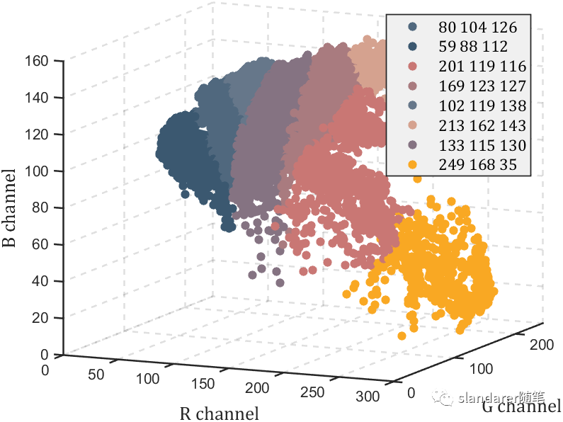
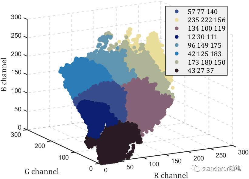
我写过一个RGB颜色统计图绘制函数：

function HistogramPic(pic)
FreqNum=zeros(size(pic,3),256);
for i=1:size(pic,3)for j=0:255FreqNum(i,j+1)=sum(sum(pic(:,:,i)==j));end
end
ax=gca;hold(ax,'on');box on;grid on
if size(FreqNum,1)==3bar(0:255,FreqNum(1,:),'FaceColor',[0.6350 0.0780 0.1840],'FaceAlpha',0.5);bar(0:255,FreqNum(2,:),'FaceColor',[0.2400 0.5300 0.0900],'FaceAlpha',0.5);bar(0:255,FreqNum(3,:),'FaceColor',[0      0.4470 0.7410],'FaceAlpha',0.5);ax.XLabel.String='RGB brightness';rrange=[num2str(min(pic(:,:,1),[],[1,2])),' , ',num2str(max(pic(:,:,1),[],[1,2]))];grange=[num2str(min(pic(:,:,2),[],[1,2])),' , ',num2str(max(pic(:,:,2),[],[1,2]))];brange=[num2str(min(pic(:,:,3),[],[1,2])),' , ',num2str(max(pic(:,:,3),[],[1,2]))];legend({['R: range[',rrange,']'],['G: range[',grange,']'],['B: range[',brange,']']},...'Location','northwest','Color',[0.9412    0.9412    0.9412],...'FontName','Cambria','LineWidth',0.8,'FontSize',11);
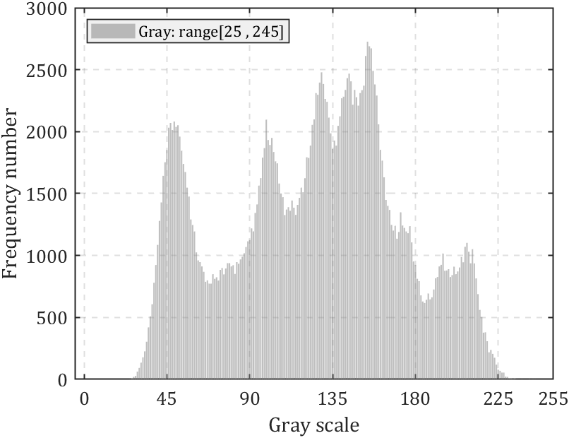
else bar(0:255,FreqNum(1,:),'FaceColor',[0.50 0.50 0.50],'FaceAlpha',0.5);ax.XLabel.String='Gray scale';krange=[num2str(min(pic(:,:,1),[],[1,2])),' , ',num2str(max(pic(:,:,1),[],[1,2]))];legend(['Gray: range[',krange,']'],...'Location','northwest','Color',[0.9412    0.9412    0.9412],...'FontName','Cambria','LineWidth',0.8,'FontSize',11);
end
ax.LineWidth=1;
ax.GridLineStyle='--';
ax.XLim=[-5 255];
ax.XTick=[0:45:255,255];
ax.YLabel.String='Frequency number';
ax.FontName='Cambria';
ax.FontSize=13;
end

非常简单的使用方法，就是读取图片后调用函数即可：

pic=imread('test.png');
HistogramPic(pic)

若图像为灰度图则效果如下：

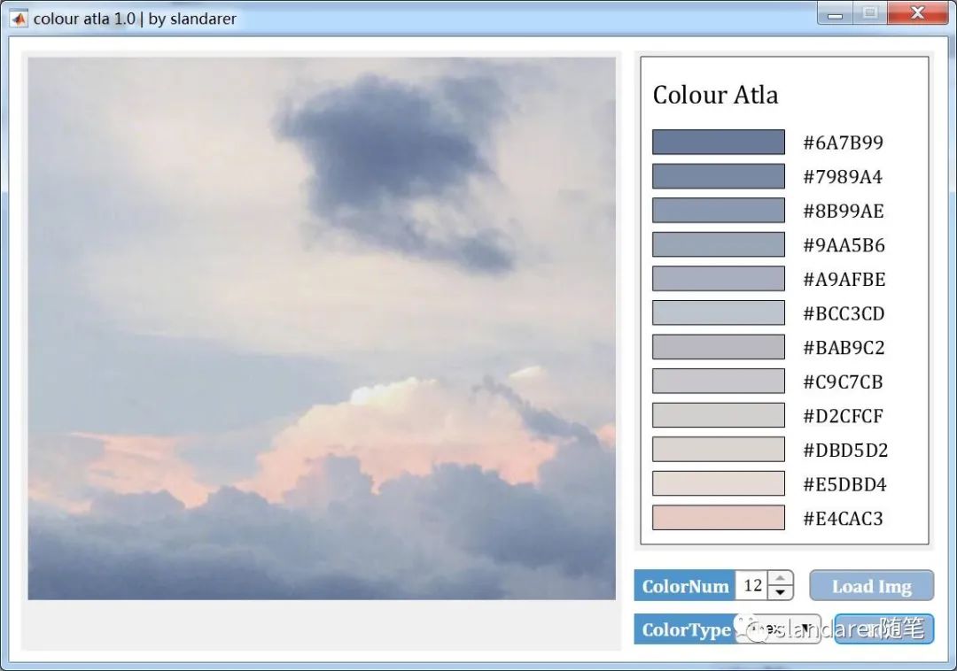
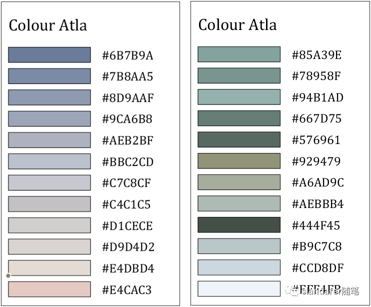
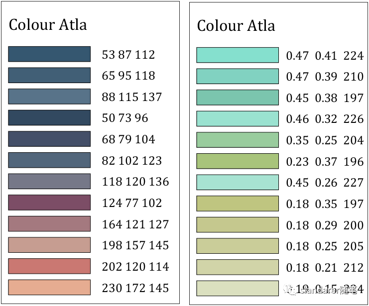
色卡生成器

从图片中提取主要颜色：https://mp.weixin.qq.com/s/Pj6t0SMDBAjQi3ecj6KVaA

颜色提取器

推荐两款颜色提取器，一款免费一款付费：

免费版：https://mp.weixin.qq.com/s/uIyvqQa9Vnz7gYLgd7lUtg

付费版：https://mp.weixin.qq.com/s/BpegP7CpOQERwrUXHexsGQ

从颜色矩阵中提取数据

之前写过一列把热图变为数值矩阵的函数，可以去瞅一眼：https://mp.weixin.qq.com/s/wzqCCFF2yvC80-ruqMKOpQ

颜色列表相关函数

颜色方块展示函数

写了个用来显示颜色的小函数：

function colorSwatches(C,sz)
ax=gca;hold on;
ax.YDir='reverse';
ax.XColor='none';
ax.YColor='none';
ax.DataAspectRatio=[1,1,1];
for i=1:sz(1)for j=1:sz(2)if j+(i-1)*sz(2)<=size(C,1)fill([-.4,-.4,.4,.4]+j,[-.4,.4,.4,-.4]+i,C(j+(i-1)*sz(2),:),...'EdgeColor','none')endend
end
end

使用方式(第一个参数是颜色列表，第二个参数是显示行列数)：

C=lines(7);
colorSwatches(C,[3,3])

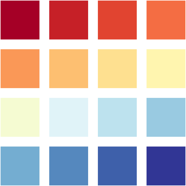
C=[0.6471         0    0.14900.7778    0.1255    0.15160.8810    0.2680    0.18950.9569    0.4275    0.26270.9804    0.5974    0.34120.9935    0.7477    0.44180.9961    0.8784    0.56470.9987    0.9595    0.68760.9595    0.9843    0.82350.8784    0.9529    0.97250.7399    0.8850    0.93330.5987    0.7935    0.88240.4549    0.6784    0.81960.3320    0.5320    0.74380.2444    0.3765    0.66540.1922    0.2118    0.5843];
colorSwatches(C,[4,4])

插值

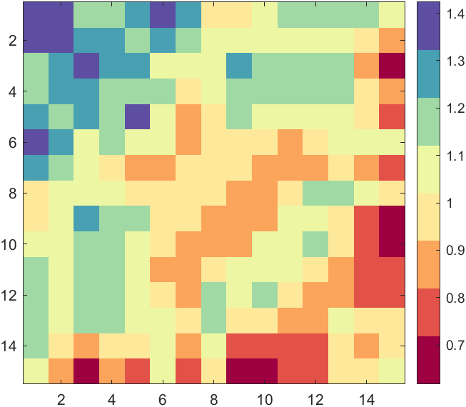
要是自己准备的颜色列表颜色数量少可能会不连续：

XData=rand(15,15);
XData=XData+XData.';
H=fspecial('average',3);
XData=imfilter(XData,H,'replicate');imagesc(XData)
CM=[0.6196    0.0039    0.25880.8874    0.3221    0.28960.9871    0.6459    0.36360.9972    0.9132    0.60340.9300    0.9720    0.63980.6319    0.8515    0.64370.2835    0.6308    0.70080.3686    0.3098    0.6353];
colormap(CM)
colorbar
hold on
ax=gca;
ax.DataAspectRatio=[1,1,1];

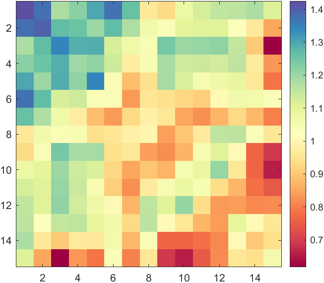
可以对其进行插值：

rng(24)
XData=rand(15,15);
XData=XData+XData.';
H=fspecial('average',3);
XData=imfilter(XData,H,'replicate');imagesc(XData)
CM=[0.6196    0.0039    0.25880.8874    0.3221    0.28960.9871    0.6459    0.36360.9972    0.9132    0.60340.9300    0.9720    0.63980.6319    0.8515    0.64370.2835    0.6308    0.70080.3686    0.3098    0.6353];
CMX=linspace(0,1,size(CM,1));
CMXX=linspace(0,1,256)';
CM=[interp1(CMX,CM(:,1),CMXX,'pchip'),interp1(CMX,CM(:,2),CMXX,'pchip'),interp1(CMX,CM(:,3),CMXX,'pchip')];
colormap(CM)
colorbar
hold on
ax=gca;
ax.DataAspectRatio=[1,1,1];

colormap编辑器

colormapeditor

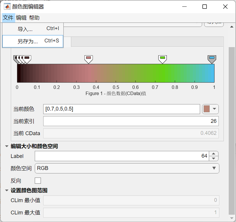
编辑完可以另存工作区，之后存为mat文件：

save CM.mat CustomColormap

之后画图就可以用啦：

rgbImage=imread("peppers.png");
imagesc(rgb2gray(rgbImage))load CM.mat
colormap(CustomColormap)

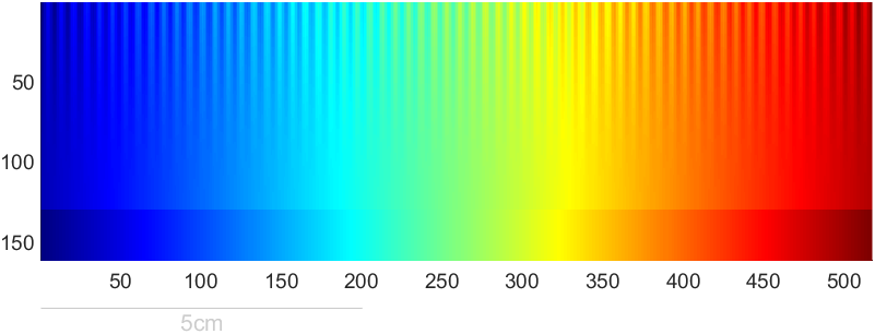
colormap显示

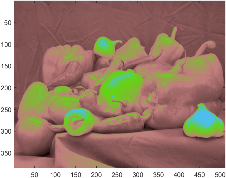
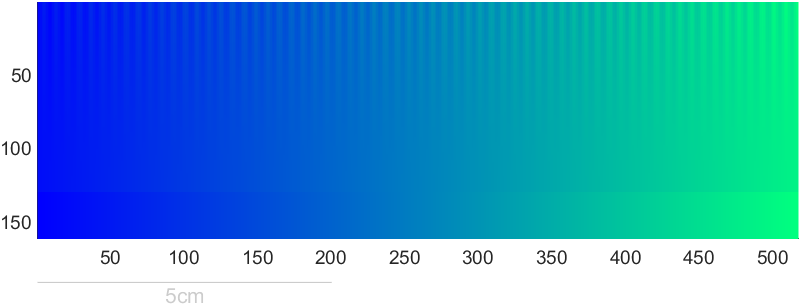
Steve Eddins大佬写了个美观的colormap展示器

Steve Eddins (2023). Colormap Test Image (https://www.mathworks.com/matlabcentral/fileexchange/63726-colormap-test-image), MATLAB Central File Exchange. 检索来源 2023/2/13.

function I = colormapTestImage(map) 
% colormapTestImage Create or display colormap test image.
%   I = colormapTestImage creates a grayscale image matrix that is useful
%   for evaluating the effectiveness of colormaps for visualizing
%   sequential data. In particular, the small-amplitude sinusoid pattern at
%   the top of the image is useful for evaluating the perceptual uniformity
%   of a colormap.
%
%   colormapTestImage(map) displays the test image using the specified
%   colormap. The colormap can be specified as the name of a colormap
%   function (such as 'parula' or 'jet'), a function handle to a colormap
%   function (such as @parula or @jet), or a P-by-3 colormap matrix.
%
%   EXAMPLES
%
%     Compute the colormap test image and save it to a file.
%
%       mk = colormapTestImage;
%       imwrite(mk,'test-image.png');
%
%     Compare the perceptual characteristics of the parula and jet
%     colormaps.
%
%       colormapTestImage('parula')
%       colormapTestImage('jet')
%
%   NOTES
%
%   The image is inspired by and adapted from the test image proposed in
%   Peter Kovesi, "Good Colour Maps: How to Design Them," CoRR, 2015,
%   https://arxiv.org/abs/1509.03700
%
%   The upper portion of the image is a linear ramp (from 0.05 to 0.95)
%   with a superimposed sinusoid. The amplitude of the sinusoid ranges from
%   0.05 at the top of the image to 0 at the bottom of the upper portion.
%
%   The lower portion of the image is a pure linear ramp from 0.0 to 1.0.
%
%   This test image differs from Kovesi's in three ways:
%
%     (a) The Kovesi test image superimposes a sinusoid on top of a
%     full-range linear ramp (0 to 1). It then rescales each row
%     independently to have full range, resulting in a linear trend slope
%     that slowly varies from row to row. The modified test image uses the
%     same linear ramp (0.05 to 0.95) on each row, with no need for
%     rescaling.
%
%     (b) The Kovesi test image has exactly 64 sinusoidal cycles
%     horizontally. This test image has 64.5 cycles plus one sample. With
%     this modification, the sinusoid is at the cycle minimum at the left
%     of the image, and it is at the cycle maximum at the right of the
%     image. With this modification, the top row of the modified test image
%     varies from exactly 0.0 on the left to exactly 1.0 on the right,
%     without rescaling.
%
%     (c) The modified test image adds to the bottom of the image a set of
%     rows containing a full-range (0.0 to 1.0) linear ramp with no
%     sinusoidal variation. That makes it easy to view how the colormap
%     appears with a full-range linear ramp.
%
%   Reference: Peter Kovesi, "Good Colour Maps: How to Design Them,"
%   CoRR, 2015, https://arxiv.org/abs/1509.03700%   Steve Eddins
%   Copyright 2017 The MathWorks, Inc.% Compare with 64 in Kovesi 2015. Adding a half-cycle here so that the ramp
% + sinusoid will be at the lowest part of the cycle on the left side of
% the image and at the highest part of the cycle on the right side of the
% image.
num_cycles = 64.5;if nargin < 1I = testImage(num_cycles);
elsedisplayTestImage(map,num_cycles)
endfunction I = testImage(num_cycles)pixels_per_cycle = 8;
A = 0.05;% Compare with width = pixels_per_cycle * num_cycles in Kovesi 2015. Here,
% the extra sample is added to fully reach the peak of the sinusoid on the
% right side of the image.
width = pixels_per_cycle * num_cycles + 1;% Determined by inspection of 
% http://peterkovesi.com/projects/colourmaps/colourmaptest.tif
height = round((width - 1) / 4);% The strategy for superimposing a varying-amplitude sinusoid on top of a
% ramp is somewhat different from Kovesi 2015. For each row of the test
% image, Kovesi adds the sinusoid to a full-range ramp and then rescales
% the row so that ramp+sinusoid is full range. A benefit of this approach
% is that each row is full range. A drawback is that the linear trend of
% each row varies as the amplitude of the superimposed sinusoid changes.
%
% Our approach here is a modification. The same linear ramp is used for
% every row of the test image, and it goes from A to 1-A, where A is the
% amplitude of the sinusoid. That way, the linear trend is identical on
% each row. The drawback is that the bottom of the test image goes from
% 0.05 to 0.95 (assuming A = 0.05) instead of from 0.00 to 1.00.
ramp = linspace(A, 1-A, width);k = 0:(width-1);
x = -A*cos((2*pi/pixels_per_cycle) * k);% Amplitude of the superimposed sinusoid varies with the square of the
% distance from the bottom of the image.
q = 0:(height-1);
y = ((height - q) / (height - 1)).^2;
I1 = (y') .* x;% Add the sinusoid to the ramp.
I = I1 + ramp;% Add region to the bottom of the image that is a full-range linear ramp.
I = [I ; repmat(linspace(0,1,width), round(height/4), 1)];function displayTestImage(map,num_cycles)name = '';
if isstring(map)map = char(map);name = map;f = str2func(map);map = f(256);
elseif ischar(map)name = map;f = str2func(map);map = f(256);
elseif isa(map,'function_handle')name = func2str(map);map = map(256);
endI = testImage(num_cycles);
[M,N] = size(I);% Display the image with a width of 2mm per cycle.
display_width_cm = num_cycles * 2 / 10;
display_height_cm = display_width_cm * M / N;fig = figure('Visible','off',...'Color','k');
fig.Units = 'centimeters';% Figure width and height will be image width and height plus 2 cm all the
% way around.
margin = 2;
fig_width = display_width_cm + 2*margin;
fig_height = display_height_cm + 2*margin;
fig.Position(3:4) = [fig_width fig_height];ax = axes('Parent',fig,...'DataAspectRatio',[1 1 1],...'YDir','reverse',...'CLim',[0 1],...'XLim',[0.5 N+0.5],...'YLim',[0.5 M+0.5]);
ax.Units = 'centimeters';
ax.Position = [margin margin display_width_cm display_height_cm];
ax.Units = 'normalized';
box(ax,'off')im = image('Parent',ax,...'CData',I,...'XData',[1 N],...'YData',[1 M],...'CDataMapping','scaled');if ~isempty(name)title(ax,name,'Color',[0.8 0.8 0.8],'Interpreter','none')
end% Draw scale line.
pixels_per_centimeter = N / (display_width_cm);
x = [0.5 5*pixels_per_centimeter];
y = (M + 30) * [1 1];
line('Parent',ax,...'XData',x,...'YData',y,...'Color',[0.8 0.8 0.8],...'Clipping','off');
text(ax,mean(x),y(1),'5cm',...'VerticalAlignment','top',...'HorizontalAlignment','center',...'Color',[0.8 0.8 0.8]);colormap(fig,map)fig.Visible = 'on';

用的时候就正常后面放颜色列表就行：

colormapTestImage(jet)

有趣实例

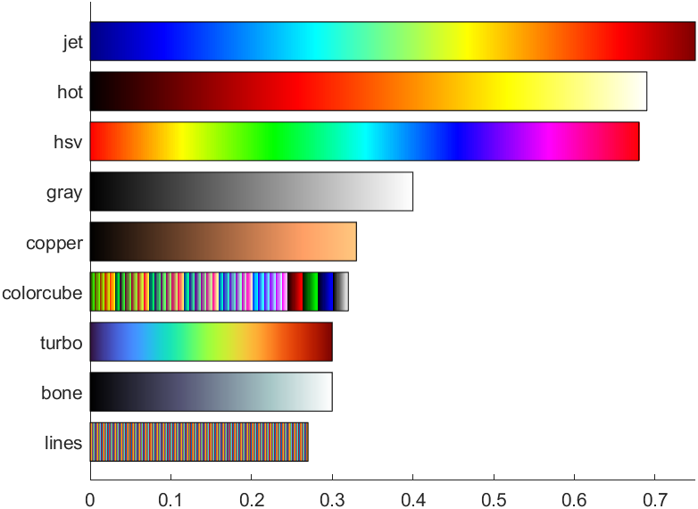
Ned Gulley大佬在迷你黑客大赛有趣的数据分析中给出的图片，展示了各种colormap使用频率排行：

https://blogs.mathworks.com/community/2022/11/08/minihack2022/?s_tid=srchtitle_minihack_1&from=cn

没提供完整代码我自己写了个：

cmaps={'jet','hot','hsv','gray','copper','colorcube','turbo','bone','lines'};
props=[.75,.69,.68,.4,.33,.32,.3,.3,.27];ax=gca;hold on
ax.XLim=[0,max(props)];
ax.YLim=[.3,1.3*length(cmaps)+1];
ax.YTick=(1:length(cmaps)).*1.3;
ax.YTickLabel=cmaps;
ax.YDir='reverse';
for i=1:length(cmaps)c=eval(cmaps{i});c=reshape(c,1,size(c,1),3);image([0,props(i)],[i,i].*1.3,c);rectangle('Position',[0 i.*1.3-.5,props(i) 1])
end

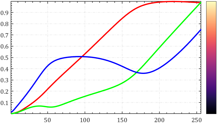
rgbplot

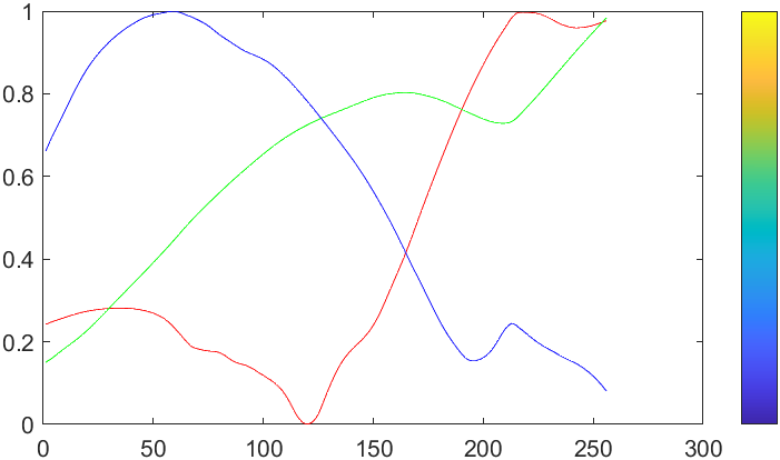
统计colormap中RGB值变化：

rgbplot(parula)
hold on
colormap(parula)
colorbar('Ticks',[])

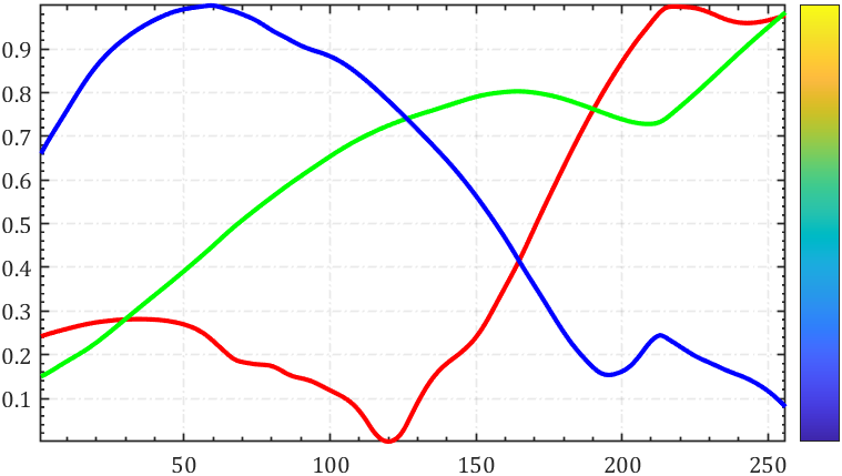
修饰一下能好看点：

rgbplot(parula)
hold on
colormap(parula)
colorbar('Ticks',[])ax=gca;hold on;axis tight
set(ax,'XMinorTick','on','YMinorTick','on','FontName','Cambria',...'XGrid','on','YGrid','on','GridLineStyle','-.','GridAlpha',.1,'LineWidth',.8);
lHdl=findobj(ax,'type','line');
for i=1:length(lHdl)lHdl(i).LineWidth=2;
end

颜色测试图表的识别

需要安装：
Image Processing Toolbox
图像处理工具箱.

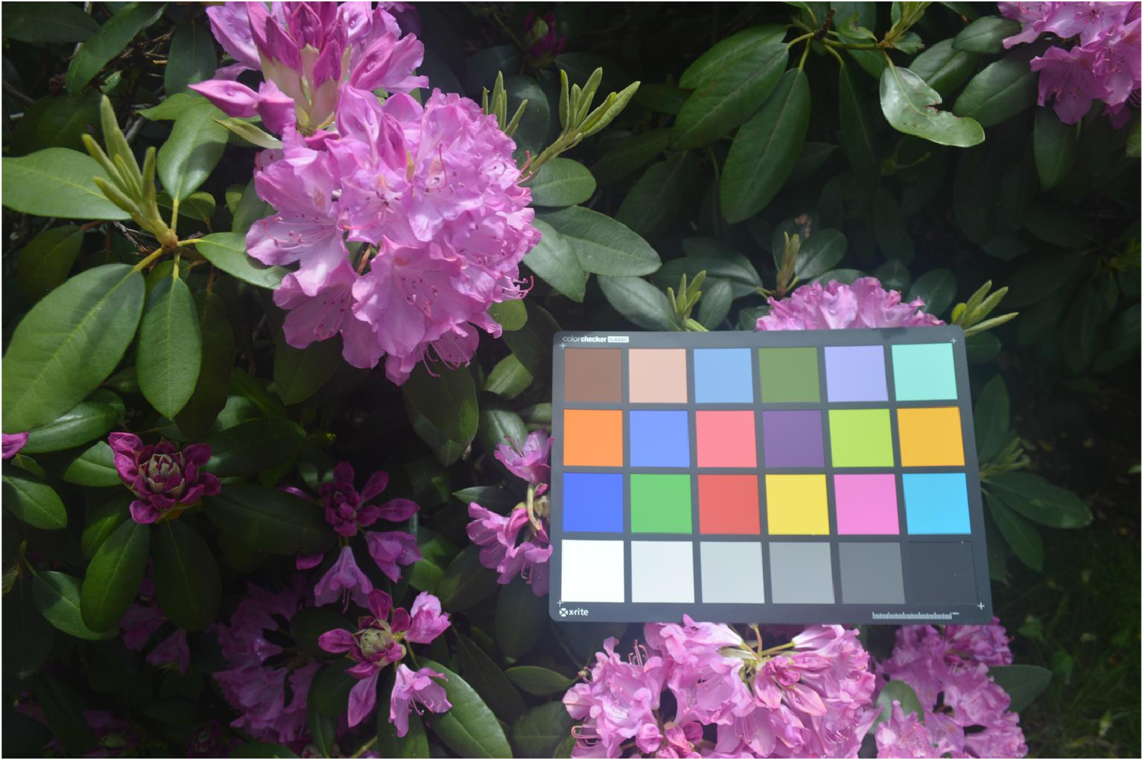
首先展示一下示例图片：

I=imread("colorCheckerTestImage.jpg");
imshow(I)

检测并进行位置标注：

chart=colorChecker(I);
displayChart(chart)

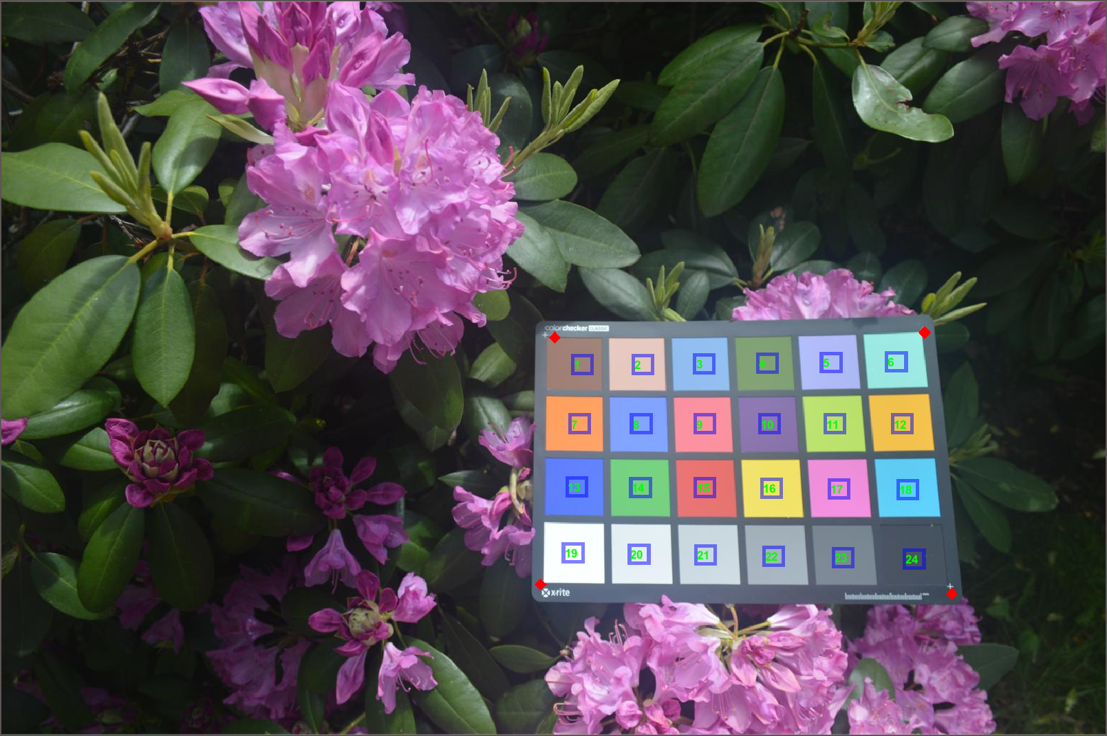
四个角点位置：

chart.RegistrationPoints

ans =
1.0e+03 *

1.3266 0.8282
0.7527 0.8147
0.7734 0.4700
1.2890 0.4632

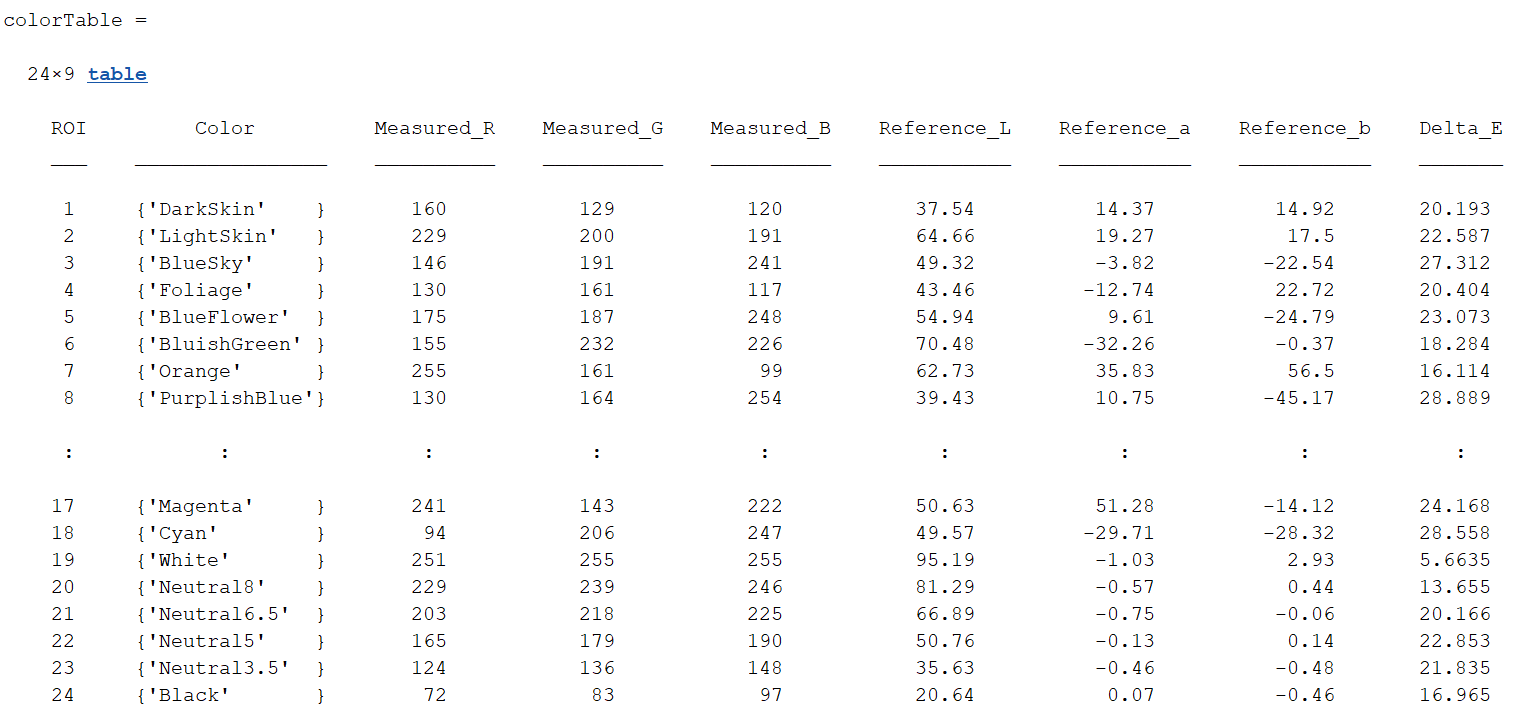
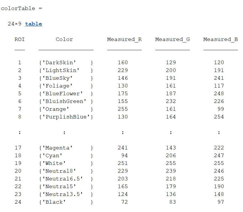
展示检测颜色：

colorTable=measureColor(chart)

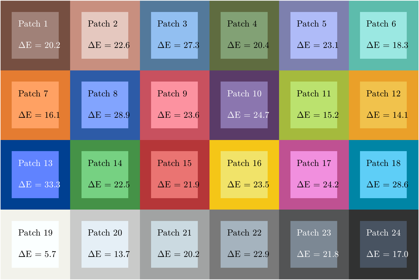
展示标准颜色和检测颜色差别：

figure
displayColorPatch(colorTable)

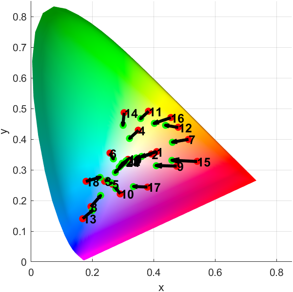
绘制CIE 1976 L* a* b*颜色空间中的测量和参考颜色对比：

figure
plotChromaticity(colorTable)