引子[1]
单摆,这个在中学物理都学过的东西,应该是非常熟悉了。
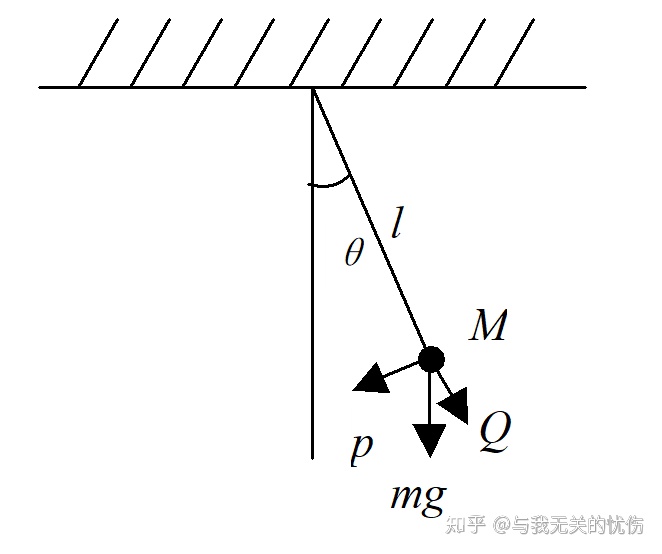
小角度简单摆
若最高处(
公式证明
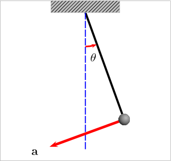
绳与对称线夹角为
由于
下面推导弹簧的周期公式(如果知道直接跳过)

设弹簧的弹性系数为
回到单摆的话题上来
刚刚推导的回复力
这是中学时候的单摆公式的推导,看得出,主要是由于条件
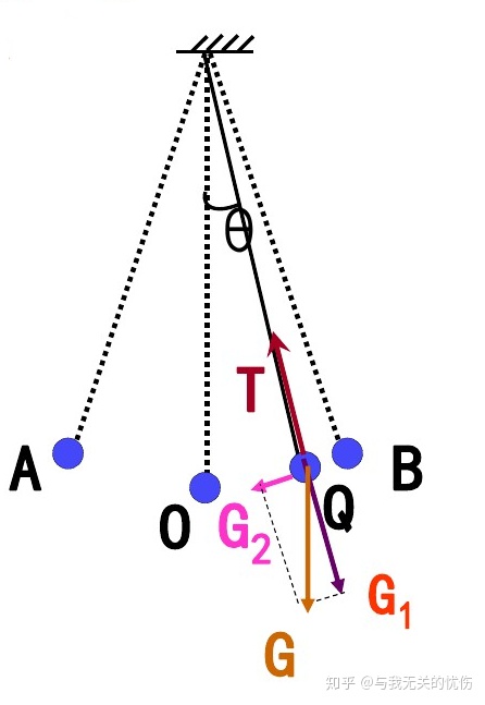
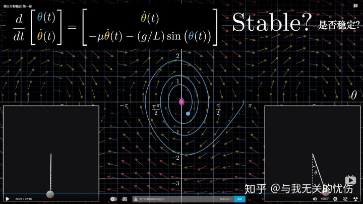
一般情况下的单摆
设与对称线的夹角为
如果
求解特殊情况,微分方程
1.猜测解法
移项
对
周期为
2.公式解法
微分方程
特征方程为
令
根据上面的结果,也可轻松知道周期为
求解一般情况,微分方程
能量守恒视角看待问题
这个方程求解比较麻烦,下面换个思路,通过能量守恒的方式来看这个问题。该系统的自由度为
从上式计算角速度
从这个式子里面可以看到,
得到式子为
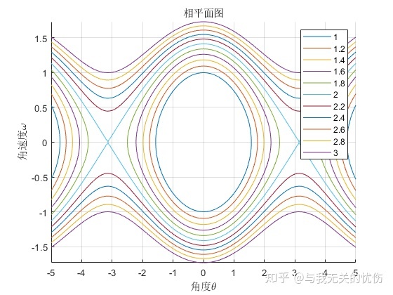
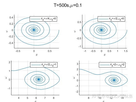
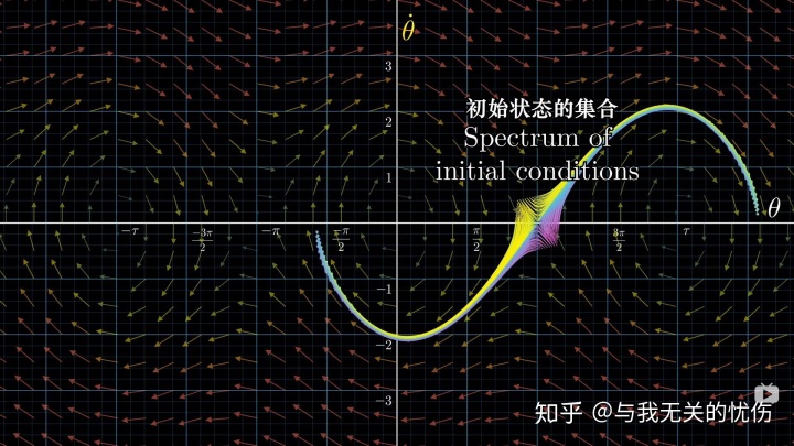
上图研究了角度与角速度之间的关系,这样的图叫做相平面图。从上面图可以看出
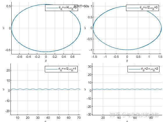
微分方程数值解法
- 图1
- 图2
- 图3
- 图4
在求解上面的微分方程的时候,使用的方法是
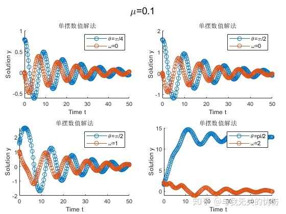
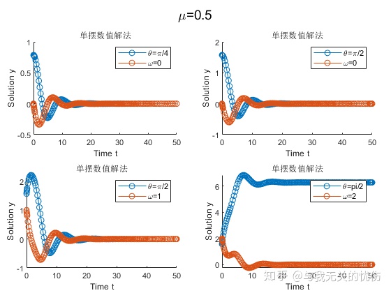
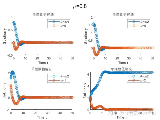
带阻尼的单摆
下面来看看带阻尼的单摆是怎么使用的其实在求解上面的代码里面就已经加入空气阻力一项了,只不过将其值设为了0,下面来看看改变这个值会发生什么。一般来说,空气阻力公式为
这里设
那么上面的微分方程变为
跟上面一样将,使用
时域图
相平面图
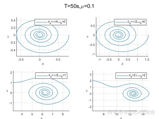
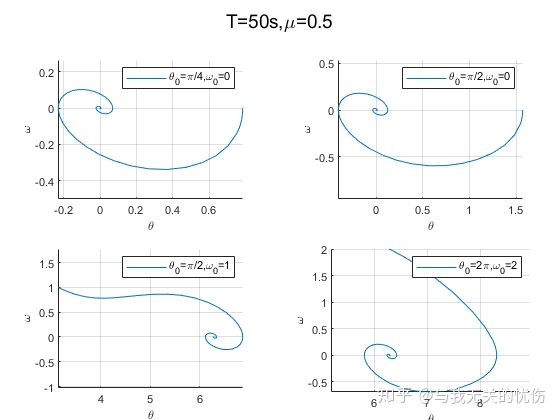
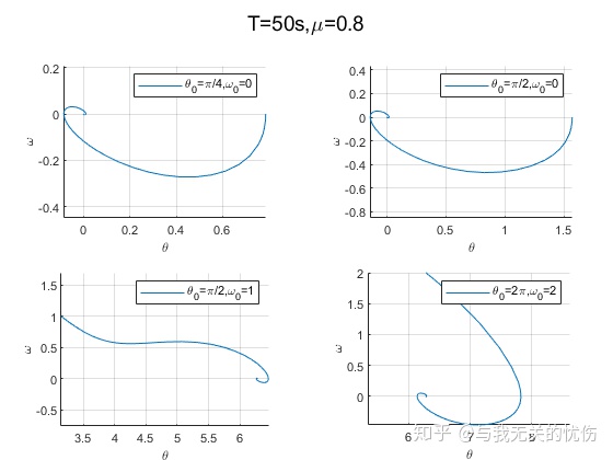
从上面这些图来看,加入空气阻力之后确实是一种带阻尼的震动图像的样子。并且阻尼越大,能量耗散的也越快。
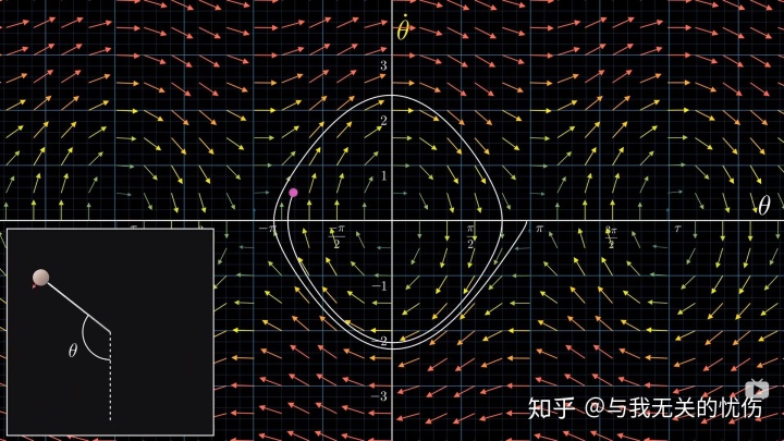
最后,其实要说的是,强烈推荐这个视频。其实前面所有讨论的东西都在下面的几张图里面了,可以回味回味。
代码
隐函数画图代码
for i=0:0.2:2
e = 1+i;
f = @(theta,theta_bar) theta_bar^2-cos(theta)-e+1;
fimplicit(f);legend(['e=',num2str(e)]);hold on;
end
xlabel('角度theta');ylabel('角速度omega');title('相平面图');
labels=num2cell(1:0.2:3);
labels = cellfun(@num2str,labels,'UniformOutput',false);
legend(labels);plotset;
print('推导函数相平面图','-dpng');
微分方程数值解代码
subplot_er(2,2,1)
[t,y] = ode45(@solve,[0,50],[pi/4,0]);
plot(y(:,1),y(:,2));
xlabel('theta');ylabel('omega');plotset;axis equal;
legend('theta_0=pi/4,omega_0=0');
subplot_er(2,2,2)
[t,y] = ode45(@solve,[0,50],[pi/2,0]);
plot(y(:,1),y(:,2));
xlabel('theta');ylabel('omega');plotset;axis equal;
legend('theta_0=pi/2,omega_0=0');
subplot_er(2,2,3)
[t,y] = ode45(@solve,[0,50],[pi,1]);
plot(y(:,1),y(:,2));
xlabel('theta');ylabel('omega');plotset;axis equal;
legend('theta_0=pi/2,omega_0=1');
subplot_er(2,2,4)
[t,y] = ode45(@solve,[0,50],[2*pi,2]);
plot(y(:,1),y(:,2));
xlabel('theta');ylabel('omega');plotset;axis equal;
legend('theta_0=2pi,omega_0=2');
suptitle('时间T=50s');
function dydt=solve(t,y)
g = 9.8;l=2*g;mu=0;
dydt = [y(2);-mu*y(2)-g/l*sin(y(1))];
end
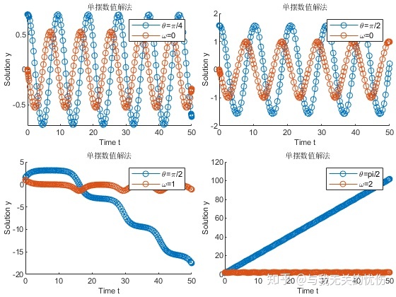
求解的时域图
subplot_er(2,2,1)
[t,y] = ode45(@solve,[0,50],[pi/4,0]);
plot(t,y(:,1),'-o',t,y(:,2),'-o');
title('单摆数值解法');xlabel('Time t');ylabel('Solution y');
legend('theta=pi/4','omega=0');
subplot_er(2,2,2)
[t,y] = ode45(@solve,[0,50],[pi/2,0]);
plot(t,y(:,1),'-o',t,y(:,2),'-o');
title('单摆数值解法');xlabel('Time t');ylabel('Solution y');
legend('theta=pi/2','omega=0');
subplot_er(2,2,3)
[t,y] = ode45(@solve,[0,50],[pi/2,1]);
plot(t,y(:,1),'-o',t,y(:,2),'-o');
title('单摆数值解法');xlabel('Time t');ylabel('Solution y');
legend('theta=pi/2','omega=1');
subplot_er(2,2,4)
[t,y] = ode45(@solve,[0,50],[pi/2,2]);
plot(t,y(:,1),'-o',t,y(:,2),'-o');
title('单摆数值解法');xlabel('Time t');ylabel('Solution y');
legend('theta=pi/2','omega=2');
function dydt=solve(t,y)
g = 9.8;l=2*g;mu=0;
dydt = [y(2);-mu*y(2)-g/l*sin(y(1))];
end
参考
- ^单摆-维基百科 https://zh.wikipedia.org/wiki/%E6%93%BA
- ^理论力学-哈工大 https://book.douban.com/subject/3866935/
- ^力学-朗道 https://book.douban.com/subject/2059252/
- ^数值方法 https://book.douban.com/subject/4780614/