1.导入包

import numpy as np
%matplotlib widget
import matplotlib.pyplot as plt
from sklearn.linear_model import LinearRegression, Ridge
from sklearn.preprocessing import StandardScaler, PolynomialFeatures
from sklearn.model_selection import train_test_split
from sklearn.metrics import mean_squared_error
import tensorflow as tf
from tensorflow.keras.models import Sequential
from tensorflow.keras.layers import Dense
from tensorflow.keras.activations import relu,linear
from tensorflow.keras.losses import SparseCategoricalCrossentropy
from tensorflow.keras.optimizers import Adamimport logging
logging.getLogger("tensorflow").setLevel(logging.ERROR)from public_tests_a1 import * tf.keras.backend.set_floatx('float64')
from assigment_utils import *tf.autograph.set_verbosity(0)

2. 评估学习算法（以线性回归为例）

在部署模型之前，如何在新数据上测试它的性能？
答案有两部分：

• 将原始数据集拆分为“训练”和“测试”集。
• 使用训练数据拟合模型参数
• 使用测试数据在新数据上评估模型
• 开发一个错误函数来评估您的模型。

2.1 分离数据集

把数据集分成测试集和训练集

# Generate some data
X,y,x_ideal,y_ideal = gen_data(18, 2, 0.7)
print("X.shape", X.shape, "y.shape", y.shape)#split the data using sklearn routine 
X_train, X_test, y_train, y_test = train_test_split(X,y,test_size=0.33, random_state=1)
print("X_train.shape", X_train.shape, "y_train.shape", y_train.shape)
print("X_test.shape", X_test.shape, "y_test.shape", y_test.shape)X.shape (18,) y.shape (18,)
X_train.shape (12,) y_train.shape (12,)
X_test.shape (6,) y_test.shape (6,)

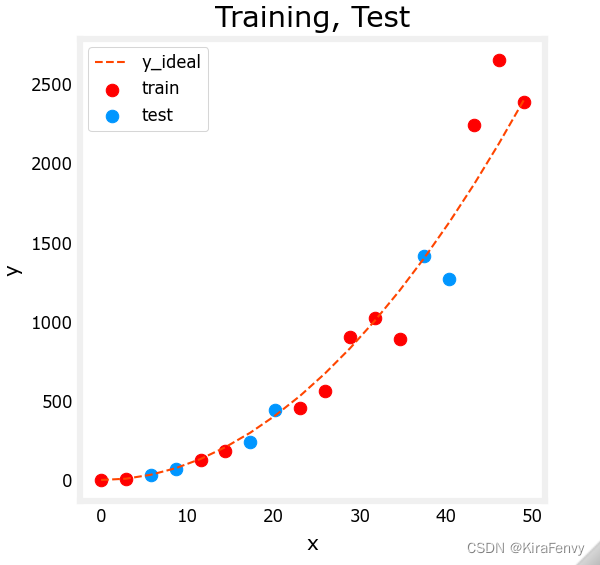
可视化数据集

fig, ax = plt.subplots(1,1,figsize=(4,4))
ax.plot(x_ideal, y_ideal, "--", color = "orangered", label="y_ideal", lw=1)
ax.set_title("Training, Test",fontsize = 14)
ax.set_xlabel("x")
ax.set_ylabel("y")ax.scatter(X_train, y_train, color = "red",           label="train")
ax.scatter(X_test, y_test,   color = dlc["dlblue"],   label="test")
ax.legend(loc='upper left')
plt.show()

2.2 误差计算

当评估线性回归模型时，将预测值和目标值的平方误差差取平均值。
$$J_{\text{test}}(\mathbf{w},b)=\frac{1}{2m_{\text{test}}}\sum _{i=0}^{m_{\text{test}}-1}(f_{\mathbf{w},b}({\mathbf{x}}_{\text{test}}^{(i)})-y_{\text{test}}^{(i)}{)}^2\text{\hspace{1em}(1)}$$

# UNQ_C1
# GRADED CELL: eval_mse
def eval_mse(y, yhat):""" Calculate the mean squared error on a data set.Args:y    : (ndarray  Shape (m,) or (m,1))  target value of each exampleyhat : (ndarray  Shape (m,) or (m,1))  predicted value of each exampleReturns:err: (scalar)             """m = len(y)err = 0.0for i in range(m):### START CODE HERE ### err_i = ((yhat[i]-y[i])**2)err += err_ierr = err /(2*m)### END CODE HERE ### return(err)#函数调用
y_hat = np.array([2.4, 4.2])
y_tmp = np.array([2.3, 4.1])
print(eval_mse(y_hat, y_tmp))

2.3 比较模型在训练集和测试集上的表现

让我们建立一个高次多项式模型来最小化训练误差。这将使用“sklearn”中的linear_regression函数。如果您想查看详细信息，代码位于导入的实用程序文件中。以下步骤为：

• 创建并拟合模型。（“fit拟合”是训练或运行梯度下降的另一个名称）。
• 计算训练数据上的误差。
• 计算测试数据的误差。

# create a model in sklearn, train on training data
degree = 10
lmodel = lin_model(degree)
lmodel.fit(X_train, y_train)# predict on training data, find training error
yhat = lmodel.predict(X_train)
err_train = lmodel.mse(y_train, yhat)# predict on test data, find error
yhat = lmodel.predict(X_test)
err_test = lmodel.mse(y_test, yhat)print(f"training err {err_train:0.2f}, test err {err_test:0.2f}")#训练集上的计算误差显著小于测试集的计算误差。
training err 58.01, test err 171215.01

为什么会发生这种情况？原因：1）过拟合，2）方差高，3）“泛化”差。1) is overfitting, 2) has high variance 3) ‘generalizes’ poorly.

def plt_train_test(X_train, y_train, X_test, y_test, x, y_pred, x_ideal, y_ideal, degree):fig, ax = plt.subplots(1,1, figsize=(4,4))fig.canvas.toolbar_visible = Falsefig.canvas.header_visible = Falsefig.canvas.footer_visible = Falseax.set_title("Poor Performance on Test Data",fontsize = 12)ax.set_xlabel("x")ax.set_ylabel("y")ax.scatter(X_train, y_train, color = "red",           label="train")ax.scatter(X_test, y_test,       color = dlc["dlblue"], label="test")ax.set_xlim(ax.get_xlim())ax.set_ylim(ax.get_ylim())ax.plot(x, y_pred,  lw=0.5, label=f"predicted, degree={degree}")ax.plot(x_ideal, y_ideal, "--", color = "orangered", label="y_ideal", lw=1)ax.legend(loc='upper left')plt.tight_layout()plt.show()# plot predictions over data range 
x = np.linspace(0,int(X.max()),100)  # predict values for plot
y_pred = lmodel.predict(x).reshape(-1,1)plt_train_test(X_train, y_train, X_test, y_test, x, y_pred, x_ideal, y_ideal, degree)

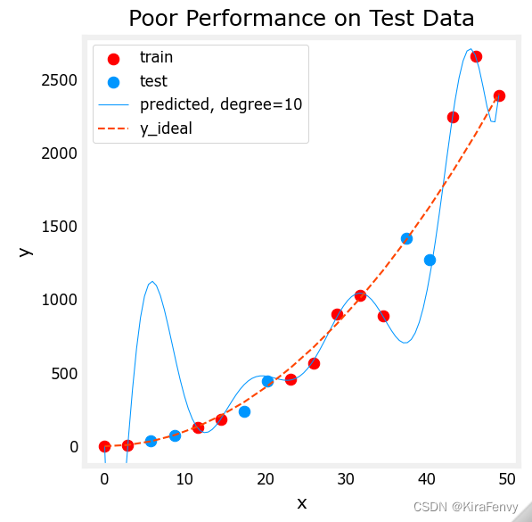
测试集错误表明此模型在新数据上无法正常工作。如果您使用测试错误来指导模型的改进，那么模型将在测试数据上表现良好……但测试数据旨在表示新数据。

您还需要另一组数据交叉验证集测试新的数据性能，来指导模型的改进

下表所示的训练、交叉验证和测试集的分布是典型的分布，但可以根据可用数据的数量而变化。

数据	占总数的百分比	说明
training	60	用于在训练或拟合中调整模型参数$w$和$b$的数据
交叉验证cross-validation	20	用于调整其他模型参数的数据，如多项式度、正则化或神经网络结构
test	20	调整后用于测试模型的数据，以衡量新数据的性能

让我们在下面生成三个数据集。我们将再次使用sklearn中的train_test_split，但将调用它两次以获得三个分割

# Generate  data
X,y, x_ideal,y_ideal = gen_data(40, 5, 0.7)
print("X.shape", X.shape, "y.shape", y.shape)#split the data using sklearn routine 
X_train, X_, y_train, y_ = train_test_split(X,y,test_size=0.40, random_state=1)
X_cv, X_test, y_cv, y_test = train_test_split(X_,y_,test_size=0.50, random_state=1)
print("X_train.shape", X_train.shape, "y_train.shape", y_train.shape)
print("X_cv.shape", X_cv.shape, "y_cv.shape", y_cv.shape)
print("X_test.shape", X_test.shape, "y_test.shape", y_test.shape)X.shape (40,) y.shape (40,)
X_train.shape (24,) y_train.shape (24,)
X_cv.shape (8,) y_cv.shape (8,)
X_test.shape (8,) y_test.shape (8,)

3.Bias and Variance

显然，多项式模型的阶数太高。你如何选择一个好的值？事实证明，如图所示，训练和交叉验证性能可以提供指导。通过尝试一系列degree values（多项式的次数值），可以评估训练和交叉验证性能。当程度变得太大时，交叉验证性能将开始相对于训练性能下降。让我们在我们的例子中尝试一下。

3.1 可视化数据集

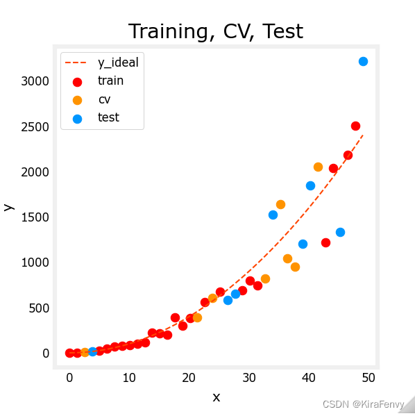
把训练集和交叉验证集可视化

fig, ax = plt.subplots(1,1,figsize=(4,4))
ax.plot(x_ideal, y_ideal, "--", color = "orangered", label="y_ideal", lw=1)
ax.set_title("Training, CV, Test",fontsize = 14)
ax.set_xlabel("x")
ax.set_ylabel("y")ax.scatter(X_train, y_train, color = "red",           label="train")
ax.scatter(X_cv, y_cv,       color = dlc["dlorange"], label="cv")
ax.scatter(X_test, y_test,   color = dlc["dlblue"],   label="test")
ax.legend(loc='upper left')
plt.show()

3.2 找到optimal degree最佳次数

在之前的实验中，您发现可以通过使用多项式创建能够拟合复杂曲线的模型（参见课程1、第2周特征工程和多项式回归实验室）。此外，您还演示了通过增加多项式的次数degree，可以创建过拟合。（参见课程1，第3周，过度装配实验室）。让我们用这些知识来测试我们区分过拟合和欠拟合的能力。

max_degree = 9
err_train = np.zeros(max_degree)    
err_cv = np.zeros(max_degree)      
# numpy.linspace()函数用于在线性空间中以均匀步长生成数字序列。
x = np.linspace(0,int(X.max()),100)  # 100表示有100个元素，前面两个值表示区间
y_pred = np.zeros((100,max_degree))  #columns are lines to plotfor degree in range(max_degree):lmodel = lin_model(degree+1)lmodel.fit(X_train, y_train)yhat = lmodel.predict(X_train)err_train[degree] = lmodel.mse(y_train, yhat)yhat = lmodel.predict(X_cv)err_cv[degree] = lmodel.mse(y_cv, yhat)y_pred[:,degree] = lmodel.predict(x)optimal_degree = np.argmin(err_cv)+1

可视化最优次数

def plt_optimal_degree(X_train, y_train, X_cv, y_cv, x, y_pred, x_ideal, y_ideal, err_train, err_cv, optimal_degree, max_degree):fig, ax = plt.subplots(1,2,figsize=(8,4))fig.canvas.toolbar_visible = Falsefig.canvas.header_visible = Falsefig.canvas.footer_visible = Falseax[0].set_title("predictions vs data",fontsize = 12)ax[0].set_xlabel("x")ax[0].set_ylabel("y")ax[0].plot(x_ideal, y_ideal, "--", color = "orangered", label="y_ideal", lw=1)ax[0].scatter(X_train, y_train, color = "red",           label="train")ax[0].scatter(X_cv, y_cv,       color = dlc["dlorange"], label="cv")ax[0].set_xlim(ax[0].get_xlim())ax[0].set_ylim(ax[0].get_ylim())for i in range(0,max_degree):ax[0].plot(x, y_pred[:,i],  lw=0.5, label=f"{i+1}")ax[0].legend(loc='upper left')ax[1].set_title("error vs degree",fontsize = 12)cpts = list(range(1, max_degree+1))ax[1].plot(cpts, err_train[0:], marker='o',label="train error", lw=2,  color = dlc["dlblue"])ax[1].plot(cpts, err_cv[0:],    marker='o',label="cv error",  lw=2, color = dlc["dlorange"])ax[1].set_ylim(*ax[1].get_ylim())ax[1].axvline(optimal_degree, lw=1, color = dlc["dlmagenta"])ax[1].annotate("optimal degree", xy=(optimal_degree,80000),xycoords='data',xytext=(0.3, 0.8), textcoords='axes fraction', fontsize=10,arrowprops=dict(arrowstyle="->", connectionstyle="arc3", color=dlc['dldarkred'], lw=1))ax[1].set_xlabel("degree")ax[1].set_ylabel("error")ax[1].legend()fig.suptitle("Find Optimal Degree",fontsize = 12)plt.tight_layout()plt.show()plt_optimal_degree(X_train, y_train, X_cv, y_cv, x, y_pred, x_ideal, y_ideal, err_train, err_cv, optimal_degree, max_degree)

上图表明，将数据分为两组，即模型训练的数据和模型未训练的数据，可以用来确定模型是欠拟合还是过拟合。在我们的示例中，我们通过增加所使用的多项式的次数，创建了从欠拟合到过拟合的各种模型。

• 在左图中，实线表示这些模型的预测。阶数为1的多项式模型生成一条与很少数据点相交的直线，而最大阶数与每个数据点非常接近。
• 右侧：
  • 训练数据上的误差（蓝色）随着模型复杂度的增加而减小
  • 交叉验证数据的误差最初随着模型开始与数据相符而减小，但随着模型开始过度拟合训练数据（未能推广）而增加。

值得注意的是，这些例子中的曲线并不像人们在课堂上画的那样平滑。很明显，分配给每组的特定数据点会显著改变你的结果。大趋势才是重要的。

3.3 Tuning Regularization调整正则化

在之前的实验中，您使用了正则化来减少过度拟合。与degree类似，可以使用相同的方法来调整正则化参数lambda（$\lambda$）。
让我们从一个高次多项式开始并改变正则化参数来证明这一点。

lambda_range = np.array([0.0, 1e-6, 1e-5, 1e-4,1e-3,1e-2, 1e-1,1,10,100])
num_steps = len(lambda_range)
degree = 10
err_train = np.zeros(num_steps)    
err_cv = np.zeros(num_steps)       
x = np.linspace(0,int(X.max()),100) 
y_pred = np.zeros((100,num_steps))  #columns are lines to plotfor i in range(num_steps):lambda_= lambda_range[i]lmodel = lin_model(degree, regularization=True, lambda_=lambda_)lmodel.fit(X_train, y_train)yhat = lmodel.predict(X_train)err_train[i] = lmodel.mse(y_train, yhat)yhat = lmodel.predict(X_cv)err_cv[i] = lmodel.mse(y_cv, yhat)y_pred[:,i] = lmodel.predict(x)optimal_reg_idx = np.argmin(err_cv) 

可视化

def plt_tune_regularization(X_train, y_train, X_cv, y_cv, x, y_pred, err_train, err_cv, optimal_reg_idx, lambda_range):fig, ax = plt.subplots(1,2,figsize=(8,4))fig.canvas.toolbar_visible = Falsefig.canvas.header_visible = Falsefig.canvas.footer_visible = Falseax[0].set_title("predictions vs data",fontsize = 12)ax[0].set_xlabel("x")ax[0].set_ylabel("y")ax[0].scatter(X_train, y_train, color = "red",           label="train")ax[0].scatter(X_cv, y_cv,       color = dlc["dlorange"], label="cv")ax[0].set_xlim(ax[0].get_xlim())ax[0].set_ylim(ax[0].get_ylim())
#   ax[0].plot(x, y_pred[:,:],  lw=0.5, label=[f"$\lambda =${i}" for i in lambda_range])for i in (0,3,7,9):ax[0].plot(x, y_pred[:,i],  lw=0.5, label=f"$\lambda =${lambda_range[i]}")ax[0].legend()ax[1].set_title("error vs regularization",fontsize = 12)ax[1].plot(lambda_range, err_train[:], label="train error", color = dlc["dlblue"])ax[1].plot(lambda_range, err_cv[:],    label="cv error",    color = dlc["dlorange"])ax[1].set_xscale('log')ax[1].set_ylim(*ax[1].get_ylim())opt_x = lambda_range[optimal_reg_idx]ax[1].vlines(opt_x, *ax[1].get_ylim(), color = "black", lw=1)ax[1].annotate("optimal lambda", (opt_x,150000), xytext=(-80,10), textcoords="offset points",arrowprops={'arrowstyle':'simple'})ax[1].set_xlabel("regularization (lambda)")ax[1].set_ylabel("error")fig.suptitle("Tuning Regularization",fontsize = 12)ax[1].text(0.05,0.44,"High\nVariance",fontsize=12, ha='left',transform=ax[1].transAxes,color = dlc["dlblue"])ax[1].text(0.95,0.44,"High\nBias",    fontsize=12, ha='right',transform=ax[1].transAxes,color = dlc["dlblue"])ax[1].legend(loc='upper left')plt.tight_layout()plt.show()plt.close("all")
plt_tune_regularization(X_train, y_train, X_cv, y_cv, x, y_pred, err_train, err_cv, optimal_reg_idx, lambda_range)

3.4 获取更多数据

当模型过拟合（高方差）时，收集额外数据可以提高性能。让我们在这里尝试一下。

def plt_tune_m(X_train, y_train, X_cv, y_cv, x, y_pred, err_train, err_cv, m_range, degree):fig, ax = plt.subplots(1,2,figsize=(8,4))fig.canvas.toolbar_visible = Falsefig.canvas.header_visible = Falsefig.canvas.footer_visible = Falseax[0].set_title("predictions vs data",fontsize = 12)ax[0].set_xlabel("x")ax[0].set_ylabel("y")ax[0].scatter(X_train, y_train, color = "red",           s=3, label="train", alpha=0.4)ax[0].scatter(X_cv, y_cv,       color = dlc["dlorange"], s=3, label="cv",    alpha=0.4)ax[0].set_xlim(ax[0].get_xlim())ax[0].set_ylim(ax[0].get_ylim())for i in range(0,len(m_range),3):ax[0].plot(x, y_pred[:,i],  lw=1, label=f"$m =${m_range[i]}")ax[0].legend(loc='upper left')ax[0].text(0.05,0.5,f"degree = {degree}", fontsize=10, ha='left',transform=ax[0].transAxes,color = dlc["dlblue"])ax[1].set_title("error vs number of examples",fontsize = 12)ax[1].plot(m_range, err_train[:], label="train error", color = dlc["dlblue"])ax[1].plot(m_range, err_cv[:],    label="cv error",    color = dlc["dlorange"])ax[1].set_xlabel("Number of Examples (m)")ax[1].set_ylabel("error")fig.suptitle("Tuning number of examples",fontsize = 12)ax[1].text(0.05,0.5,"High\nVariance",        fontsize=12, ha='left',transform=ax[1].transAxes,color = dlc["dlblue"])ax[1].text(0.95,0.5,"Good \nGeneralization", fontsize=12, ha='right',transform=ax[1].transAxes,color = dlc["dlblue"])ax[1].legend()plt.tight_layout()plt.show()  X_train, y_train, X_cv, y_cv, x, y_pred, err_train, err_cv, m_range,degree = tune_m()
plt_tune_m(X_train, y_train, X_cv, y_cv, x, y_pred, err_train, err_cv, m_range, degree)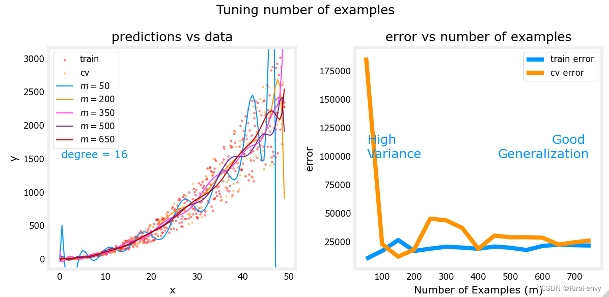

上面的图表显示，当模型具有高方差且过度拟合时，添加更多示例可以提高性能。注意左图上的曲线。最高值为$m$的最终曲线是位于数据中心的平滑曲线。在右边，随着示例数量的增加，训练集和交叉验证集的性能收敛到相似的值。请注意，曲线并不像你在课堂上看到的那样平滑。趋势依然清晰：更多的数据有助于泛化generalization。

请注意，当模型具有高偏差（欠拟合）时，添加更多示例并不能提高性能。

4.评估学习算法（神经网络）

4.1 数据集（聚类问题）

运行下面的单元格以生成数据集，并将其拆分为训练集、交叉验证（CV）和测试集。在本例中，我们增加了交叉验证数据点的百分比，以供强调。

# Generate and split data set
X, y, centers, classes, std = gen_blobs()# split the data. Large CV population for demonstration
X_train, X_, y_train, y_ = train_test_split(X,y,test_size=0.50, random_state=1)
X_cv, X_test, y_cv, y_test = train_test_split(X_,y_,test_size=0.20, random_state=1)
print("X_train.shape:", X_train.shape, "X_cv.shape:", X_cv.shape, "X_test.shape:", X_test.shape)X_train.shape: (400, 2) X_cv.shape: (320, 2) X_test.shape: (80, 2)

可视化数据：

def plt_mc_data(ax, X, y, classes,  class_labels=None, map=plt.cm.Paired, legend=False,size=50, m='o'):for i in range(classes):idx = np.where(y == i)col = len(idx[0])*[i]label = class_labels[i] if class_labels else "c{}".format(i)ax.scatter(X[idx, 0], X[idx, 1],  marker=m,c=col, vmin=0, vmax=map.N, cmap=map,s=size, label=label)if legend: ax.legend()ax.axis('equal')def plt_train_eq_dist(X_train,y_train,classes, X_cv,   y_cv, centers, std):css = np.unique(y_train)fig,ax = plt.subplots(1,2,figsize=(8,4))fig.canvas.toolbar_visible = Falsefig.canvas.header_visible = Falsefig.canvas.footer_visible = Falseplt_mc_data(ax[0], X_train,y_train,classes, map=dkcolors_map, legend=True, size=50)plt_mc_data(ax[0], X_cv,   y_cv,   classes, map=ltcolors_map, legend=True, m="<")ax[0].set_title("Training, CV Data")for c in css:circ = plt.Circle(centers[c], 2*std, color=dkcolors_map(c), clip_on=False, fill=False, lw=0.5)ax[0].add_patch(circ)plt_train_eq_dist(X_train, y_train,classes, X_cv, y_cv, centers, std)

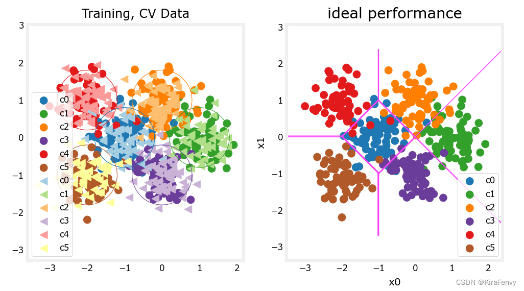
上面，你可以看到左边的数据。有六个按颜色识别的簇。显示了训练点（点）和交叉验证点（三角形）。有趣的点是那些位于不明确位置的点，其中任何一个集群都可能认为它们是成员。你希望神经网络模型能做什么？过度拟合的例子是什么？填充不足？

右边是一个“理想”模型的例子，或者一个知道数据来源的模型。这些线表示“等距”边界，其中中心点之间的距离相等。值得注意的是，该模型将“错误分类”总数据集的大约8%。

4.2 计算分类误差评估分类模型

The evaluation function for categorical models used here is simply the fraction of incorrect predictions:
$$J_{cv}=\frac{1}{m}\sum _{i=0}^{m-1}\{\begin{array}{ll}1,& \text{if y^(i)=y(i)}\\ 0,& \text{otherwise}\end{array}$$

下面，完成计算分类错误的例程。注意，在这个实验室中，目标值是类别的索引，而不是独热编码.

# UNQ_C2
# GRADED CELL: eval_cat_err
def eval_cat_err(y, yhat):""" Calculate the categorization errorArgs:y    : (ndarray  Shape (m,) or (m,1))  target value of each exampleyhat : (ndarray  Shape (m,) or (m,1))  predicted value of each exampleReturns:|cerr: (scalar)             """m = len(y)incorrect = 0for i in range(m):### START CODE HERE ### if y[i]!=yhat[i]:incorrect+=1cerr = incorrect / ### END CODE HERE ### return(cerr)

检查并调用函数：

squeeze函数：从数组的形状中删除单维度条目，即把shape中为1的维度去掉
语法：numpy.squeeze(a, axis = None)
1）a表示输入的数组；
2）axis用于指定需要删除的维度，但是指定的维度必须为单维度，否则将会报错；
3）axis的取值可为None 或 int 或 tuple of ints, 可选。若axis为空，则删除所有单维度的条目；
4）返回值：数组
5) 不会修改原数组

y_hat = np.array([1, 2, 0])
y_tmp = np.array([1, 2, 3])
print(f"categorization error {np.squeeze(eval_cat_err(y_hat, y_tmp)):0.3f}, expected:0.333" )
y_hat = np.array([[1], [2], [0], [3]])
y_tmp = np.array([[1], [2], [1], [3]])
print(f"categorization error {np.squeeze(eval_cat_err(y_hat, y_tmp)):0.3f}, expected:0.250" )

5.模型复杂度

下面，您将构建两个模型。复杂模型和简单模型。您将对模型进行评估，以确定它们是否可能过拟合或欠拟合

5.1 构建复杂模型

Below, compose a three-layer model:

• Dense layer with 120 units, relu activation
• Dense layer with 40 units, relu activation
• Dense layer with 6 units and a linear activation (not softmax)
  Compile using
• loss with SparseCategoricalCrossentropy, remember to use from_logits=True
• Adam optimizer with learning rate of 0.01.

# UNQ_C3
# GRADED CELL: model
import logging
logging.getLogger("tensorflow").setLevel(logging.ERROR)tf.random.set_seed(1234)
model = Sequential([### START CODE HERE ### Dense(120, activation = "relu", name = "L1"),Dense(40, activation = "relu", name = "L2"),Dense(classes, activation = "linear", name = "L3"),### END CODE HERE ### ], name="Complex"
)
model.compile(### START CODE HERE ### loss=tf.keras.losses.SparseCategoricalCrossentropy(from_logits=True),optimizer=tf.keras.optimizers.Adam(0.01),### END CODE HERE ### 
)# BEGIN UNIT TEST
model.fit(X_train, y_train,epochs=200
)
# END UNIT TESTmodel.summary()Model: "Complex"
_________________________________________________________________Layer (type)                Output Shape              Param #   
=================================================================L1 (Dense)                  (None, 120)               360       L2 (Dense)                  (None, 40)                4840      L3 (Dense)                  (None, 6)                 246       =================================================================
Total params: 5,446
Trainable params: 5,446
Non-trainable params: 0

画图描述预测结果

#Plot a multi-class categorical decision boundary
# This version handles a non-vector prediction (adds a for-loop over points)
def plot_cat_decision_boundary(ax, X,predict , class_labels=None, legend=False, vector=True, color='g', lw = 1):# create a mesh to points to plotpad = 0.5x_min, x_max = X[:, 0].min() - pad, X[:, 0].max() + pady_min, y_max = X[:, 1].min() - pad, X[:, 1].max() + padh = max(x_max-x_min, y_max-y_min)/200xx, yy = np.meshgrid(np.arange(x_min, x_max, h),np.arange(y_min, y_max, h))points = np.c_[xx.ravel(), yy.ravel()]#print("points", points.shape)#make predictions for each point in meshif vector:Z = predict(points)else:Z = np.zeros((len(points),))for i in range(len(points)):Z[i] = predict(points[i].reshape(1,2))Z = Z.reshape(xx.shape)#contour plot highlights boundaries between values - classes in this caseax.contour(xx, yy, Z, colors=color, linewidths=lw) ax.axis('tight')def plt_nn(model_predict,X_train,y_train, classes, X_cv, y_cv, suptitle=""):#plot the decison boundary.fig,ax = plt.subplots(1,2, figsize=(8,4))fig.canvas.toolbar_visible = Falsefig.canvas.header_visible = Falsefig.canvas.footer_visible = Falseplot_cat_decision_boundary(ax[0], X_train, model_predict,  vector=True)ax[0].set_title("training data", fontsize=14)#add the original data to the decison boundaryplt_mc_data(ax[0], X_train,y_train, classes, map=dkcolors_map, legend=True, size=75)ax[0].set_xlabel('x0') ; ax[0].set_ylabel("x1");plot_cat_decision_boundary(ax[1], X_train, model_predict,  vector=True)ax[1].set_title("cross-validation data", fontsize=14)plt_mc_data(ax[1], X_cv,y_cv, classes, map=ltcolors_map, legend=True, size=100, m='<')ax[1].set_xlabel('x0') ; ax[1].set_ylabel("x1"); fig.suptitle(suptitle,fontsize = 12)plt.show()#make a model for plotting routines to call
model_predict = lambda Xl: np.argmax(tf.nn.softmax(model.predict(Xl)).numpy(),axis=1)
plt_nn(model_predict,X_train,y_train, classes, X_cv, y_cv, suptitle="Complex Model")

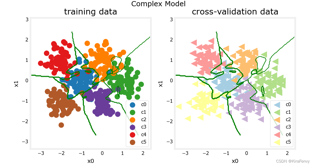
计算分类误差：

training_cerr_complex = eval_cat_err(y_train, model_predict(X_train))
cv_cerr_complex = eval_cat_err(y_cv, model_predict(X_cv))
print(f"categorization error, training, complex model: {training_cerr_complex:0.3f}")
print(f"categorization error, cv,       complex model: {cv_cerr_complex:0.3f}")categorization error, training, complex model: 0.007
categorization error, cv,       complex model: 0.100

5.2 构建简单模型

# UNQ_C4
# GRADED CELL: model_stf.random.set_seed(1234)
model_s = Sequential([### START CODE HERE ### Dense(classes,activation="relu",name="L1"),Dense(classes,activation="linear",name="L2"),### END CODE HERE ### ], name = "Simple"
)
model_s.compile(### START CODE HERE ### loss=tf.keras.losses.SparseCategoricalCrossentropy(from_logits = True),optimizer=tf.keras.optimizers.Adam(learning_rate=0.01),### START CODE HERE ### 
)# BEGIN UNIT TEST
model_s.summary()Model: "Simple"
_________________________________________________________________Layer (type)                Output Shape              Param #   
=================================================================L1 (Dense)                  (None, 6)                 18        L2 (Dense)                  (None, 6)                 42        =================================================================
Total params: 60
Trainable params: 60

计算分类错误（使用前面写过的函数）

training_cerr_simple = eval_cat_err(y_train, model_predict_s(X_train))
cv_cerr_simple = eval_cat_err(y_cv, model_predict_s(X_cv))
print(f"categorization error, training, simple model, {training_cerr_simple:0.3f}, complex model: {training_cerr_complex:0.3f}" )
print(f"categorization error, cv,       simple model, {cv_cerr_simple:0.3f}, complex model: {cv_cerr_complex:0.3f}" )

6.正则化

首先依然先构建拟合模型

# UNQ_C5
# GRADED CELL: model_rtf.random.set_seed(1234)
model_r = Sequential([### START CODE HERE ### Dense(120,activation = "relu",name = "L1"),Dense(40,activation = "relu",name = "L2"),Dense(6,activation = "linear",name = "L3")### START CODE HERE ### ], name=“ComplexRegularized”
)
model_r.compile(### START CODE HERE ### loss=tf.keras.losses.SparseCategoricalCrossentropy(from_logits=True),optimizer=tf.keras.optimizers.Adam(learning_rate=0.01)### START CODE HERE ### 
)# BEGIN UNIT TEST
model_r.fit(X_train, y_train,epochs=1000
)
# END UNIT TEST

然后

#make a model for plotting routines to call
model_predict_r = lambda Xl: np.argmax(tf.nn.softmax(model_r.predict(Xl)).numpy(),axis=1)plt_nn(model_predict_r, X_train,y_train, classes, X_cv, y_cv, suptitle="Regularized")

training_cerr_reg = eval_cat_err(y_train, model_predict_r(X_train))
cv_cerr_reg = eval_cat_err(y_cv, model_predict_r(X_cv))
test_cerr_reg = eval_cat_err(y_test, model_predict_r(X_test))
print(f"categorization error, training, regularized: {training_cerr_reg:0.3f}, simple model, {training_cerr_simple:0.3f}, complex model: {training_cerr_complex:0.3f}" )
print(f"categorization error, cv,       regularized: {cv_cerr_reg:0.3f}, simple model, {cv_cerr_simple:0.3f}, complex model: {cv_cerr_complex:0.3f}" )

正则化后的error计算：

training_cerr_reg = eval_cat_err(y_train, model_predict_r(X_train))
cv_cerr_reg = eval_cat_err(y_cv, model_predict_r(X_cv))
test_cerr_reg = eval_cat_err(y_test, model_predict_r(X_test))
print(f"categorization error, training, regularized: {training_cerr_reg:0.3f}, simple model, {training_cerr_simple:0.3f}, complex model: {training_cerr_complex:0.3f}" )
print(f"categorization error, cv,       regularized: {cv_cerr_reg:0.3f}, simple model, {cv_cerr_simple:0.3f}, complex model: {cv_cerr_complex:0.3f}" )categorization error, training, regularized: 0.005, simple model, 0.077, complex model: 0.035
categorization error, cv,       regularized: 0.106, simple model, 0.062, complex model: 0.116

7、多次训练寻找最优的正则化系数

tf.random.set_seed(1234)
lambdas = [0.0, 0.001, 0.01, 0.05, 0.1, 0.2, 0.3]
models=[None] * len(lambdas)
for i in range(len(lambdas)):lambda_ = lambdas[i]models[i] =  Sequential([Dense(120, activation = 'relu', kernel_regularizer=tf.keras.regularizers.l2(lambda_)),Dense(40, activation = 'relu', kernel_regularizer=tf.keras.regularizers.l2(lambda_)),Dense(classes, activation = 'linear')])models[i].compile(loss=tf.keras.losses.SparseCategoricalCrossentropy(from_logits=True),optimizer=tf.keras.optimizers.Adam(0.01),)models[i].fit(X_train,y_train,epochs=1000)print(f"Finished lambda = {lambda_}")

画图迭代图：

def plot_iterate(lambdas, models, X_train, y_train, X_cv, y_cv):err_train = np.zeros(len(lambdas))err_cv = np.zeros(len(lambdas))for i in range(len(models)):err_train[i] = eval_cat_err(y_train,np.argmax( models[i](X_train), axis=1))err_cv[i] = eval_cat_err(y_cv, np.argmax( models[i](X_cv), axis=1))fig, ax = plt.subplots(1,1,figsize=(6,4))fig.canvas.toolbar_visible = Falsefig.canvas.header_visible = Falsefig.canvas.footer_visible = Falseax.set_title("error vs regularization",fontsize = 12)ax.plot(lambdas, err_train, marker='o', label="train error", color = dlc["dlblue"])ax.plot(lambdas, err_cv,    marker='o', label="cv error",    color = dlc["dlorange"])ax.set_xscale('log')ax.set_ylim(*ax.get_ylim())ax.set_xlabel("Regularization (lambda)",fontsize = 14)ax.set_ylabel("Error",fontsize = 14)ax.legend()fig.suptitle("Tuning Regularization",fontsize = 14)ax.text(0.05,0.14,"Training Error\nlower than CV",fontsize=12, ha='left',transform=ax.transAxes,color = dlc["dlblue"])ax.text(0.95,0.14,"Similar\nTraining, CV",    fontsize=12, ha='right',transform=ax.transAxes,color = dlc["dlblue"])plt.show()plot_iterate(lambdas, models, X_train, y_train, X_cv, y_cv)

随着正则化系数的增加，模型在训练和交叉验证数据集上的性能会收敛。对于这个数据集和模型，lambda>0.01似乎是一个合理的选择。

7.测试

复杂、简单模型以及理想模型的对比：

def plt_compare(X,y, classes, simple, regularized, centers):plt.close("all")fig,ax = plt.subplots(1,3, figsize=(8,3))fig.canvas.toolbar_visible = Falsefig.canvas.header_visible = Falsefig.canvas.footer_visible = False#plt simple   plot_cat_decision_boundary(ax[0], X, simple,  vector=True)ax[0].set_title("Simple Model", fontsize=14)plt_mc_data(ax[0], X,y, classes, map=dkcolors_map, legend=True, size=75)ax[0].set_xlabel('x0') ; ax[0].set_ylabel("x1");#plt regularized   plot_cat_decision_boundary(ax[1], X, regularized,  vector=True)ax[1].set_title("Regularized Model", fontsize=14)plt_mc_data(ax[1], X,y, classes, map=dkcolors_map, legend=True, size=75)ax[1].set_xlabel('x0') ; ax[0].set_ylabel("x1");#plt idealcat_predict = lambda pt: recat(pt.reshape(1,2), centers)plot_cat_decision_boundary(ax[2], X, cat_predict,  vector=False)ax[2].set_title("Ideal Model", fontsize=14)plt_mc_data(ax[2], X,y, classes, map=dkcolors_map, legend=True, size=75)ax[2].set_xlabel('x0') ; ax[0].set_ylabel("x1");err_s = eval_cat_err(y, simple(X))err_r = eval_cat_err(y, regularized(X))ax[0].text(-2.75,3,f"err_test={err_s:0.2f}", fontsize=12)ax[1].text(-2.75,3,f"err_test={err_r:0.2f}", fontsize=12)m = len(X)y_eq  = np.zeros(m)for i in range(m):y_eq[i] = recat(X[i], centers)err_eq = eval_cat_err(y, y_eq)ax[2].text(-2.75,3,f"err_test={err_eq:0.2f}", fontsize=12)plt.show()plt_compare(X_test,y_test, classes, model_predict_s, model_predict_r, centers)

8.总结

• 将数据拆分为训练集和未训练集可以区分欠拟合和过拟合

• 创建三个数据集：培训、交叉验证和测试，您可以

• 使用训练集训练参数$W、B$

• 使用交叉验证集调整模型参数，如复杂性、正则化和示例数量

• 使用测试集评估您的“真实世界”性能。

• 将训练与交叉验证性能进行比较，可以深入了解模型过度拟合（高方差）或欠拟合（高偏差）的倾向

9.课后题

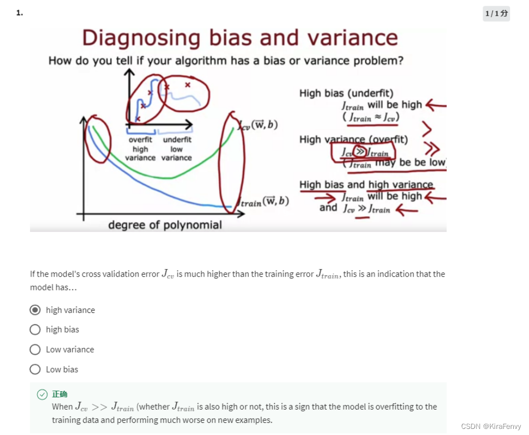
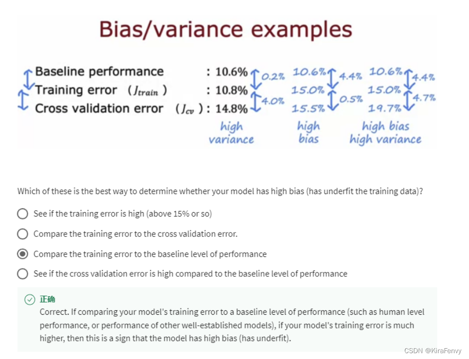
9.1.识别bias和variance

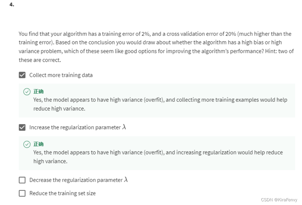
9.2 解决高bias和variance

碰到高bias的解决办法：调低lambda、收集更多数据添加多项式特征（交互特征

交互特征（多项式特征）

交互特征可以对线性模型进行扩展，使之包含输入特征的两两组合，捕获特征之间的交互作用），对线性模型有很大的提升，但对于更复杂的模型，如核SVM，随机森林，则意义不大。

碰到高variance：收集更多训练数据，调低lambda

9.3 概念

错误分析

手动检查模型错误分类的训练示例样本，以确定常见特征和趋势。
通过识别类似类型的错误，您可以收集更多类似于这些错误分类示例的数据，以便训练模型改进这些类型的示例。

数据增强

我们有时会取一个现有的训练示例并对其进行修改（例如，通过稍微旋转图像）创建具有相同标签的新示例，这个过程就是数据增强

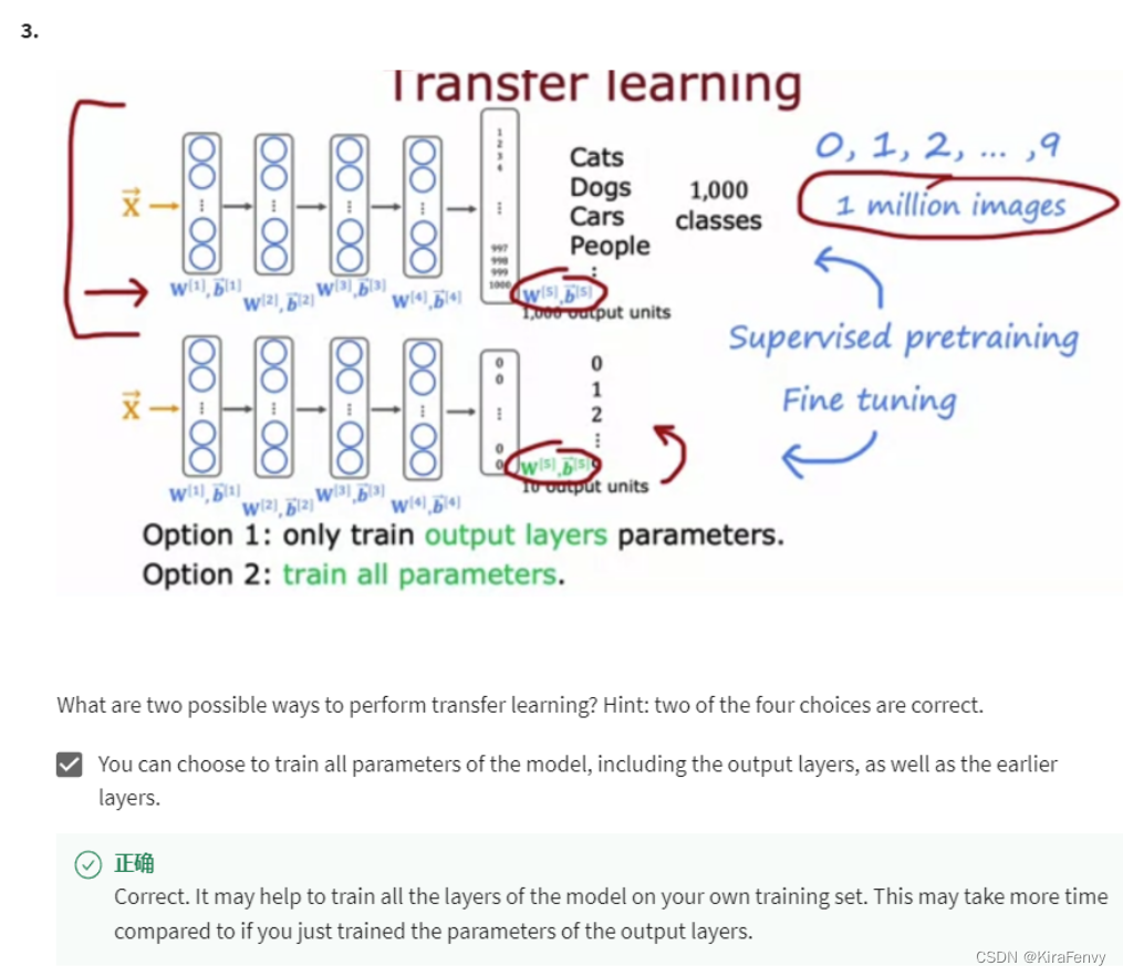
迁移学习

您可以选择训练模型的所有参数，包括输出层以及之前的层。这可能有助于在自己的训练集上训练模型的所有层。这可能需要更多时间相比只是训练了输出层的参数。

可以选择只训练输出层的参数，而不训练模型的其他参数。模型的早期层可以按原样重用，因为它们识别的是低层

迁移学习就是pre-train + fine-tune，什么是预训练和微调？
你需要搭建一个网络模型来完成一个特定的图像分类的任务。首先，你需要随机初始化参数，然后开始训练网络，不断调整直到网络的损失越来越小。在训练的过程中，一开始初始化的参数会不断变化。当你觉得结果很满意的时候，你就可以将训练模型的参数保存下来，以便训练好的模型可以在下次执行类似任务时获得较好的结果。这个过程就是 pre-training。
之后，你又接收到一个类似的图像分类的任务。这时候，你可以直接使用之前保存下来的模型的参数来作为这一任务的初始化参数，然后在训练的过程中，依据结果不断进行一些修改。这时候，你使用的就是一个 pre-trained 模型，而过程就是 fine-tuning。